

Abstract
Global-scale hydrological models are routinely used to assess water scarcity, flood hazards and droughts worldwide. Recent efforts to incorporate anthropogenic activities in these models have enabled more realistic comparisons with observations. Here we evaluate simulations from an ensemble of six models participating in the second phase of the Inter-Sectoral Impact Model Inter-comparison Project (ISIMIP2a). We simulate monthly runoff in 40 catchments, spatially distributed across eight global hydrobelts. The performance of each model and the ensemble mean is examined with respect to their ability to replicate observed mean and extreme runoff under human-influenced conditions. Application of a novel integrated evaluation metric to quantify the models' ability to simulate timeseries of monthly runoff suggests that the models generally perform better in the wetter equatorial and northern hydrobelts than in drier southern hydrobelts. When model outputs are temporally aggregated to assess mean annual and extreme runoff, the models perform better. Nevertheless, we find a general trend in the majority of models towards the overestimation of mean annual runoff and all indicators of upper and lower extreme runoff. The models struggle to capture the timing of the seasonal cycle, particularly in northern hydrobelts, while in southern hydrobelts the models struggle to reproduce the magnitude of the seasonal cycle. It is noteworthy that over all hydrological indicators, the ensemble mean fails to perform better than any individual model—a finding that challenges the commonly held perception that model ensemble estimates deliver superior performance over individual models. The study highlights the need for continued model development and improvement. It also suggests that caution should be taken when summarising the simulations from a model ensemble based upon its mean output.
Export citation and abstract BibTeX RIS

Original content from this work may be used under the terms of the Creative Commons Attribution 3.0 licence.
Any further distribution of this work must maintain attribution to the author(s) and the title of the work, journal citation and DOI.
1. Introduction
Global hydrological models (GHMs) and land surface models (LSMs) are used for assessing the impacts of climate change on water availability and scarcity [1–5], droughts [6, 7], flood hazard and risk [8–11], the response of the global hydrological cycle to climate change mitigation [12], forecasting at short timescales [13] and examining the role of water in assessments of food security [14–16]. In turn, their results are used to inform global policy decisions on climate change [17, 18]. Therefore, it is important to understand the strengths and limitations of these models in simulating global hydrological variability.
The aims of this study are to: provide new understanding on how global-scale hydrological models perform in different hydro-geographical locations of the globe; to highlight the current strengths and limitations of global-scale hydrological modelling; to identify opportunities for the community to improve the models; and to explore the potential implications of our research for future work in the field.
Previous global evaluation studies (table 1) differ from each other in several ways: in the number of models evaluated (2–14, with a median of 6); the number of catchments included (8–6192); the size of catchments considered (10 km2–4 758 000 km2); the evaluation metrics calculated; the hydrological indicators evaluated; and the period of analyses. The highly varied approaches taken in previous studies means there remain several opportunities for improving the way in which model evaluation studies are conducted.
Table 1. Overview of selected global-scale studies evaluating multiple models, including the present study. GHM: Global Hydrological Model, LSM: Land Surface Model, DGVM: Dynamic Global Vegetation Model, GCM: Global Climate Model, MAR: mean annual runoff/discharge, MMR: mean monthly runoff/discharge and/or seasonality, MDR: mean daily runoff/discharge, HFP: extreme high flow percentiles (e.g. Q5), LFP: extreme low flow percentiles (e.g. Q95), HFR: high flow return periods, LFR: low flow return periods.
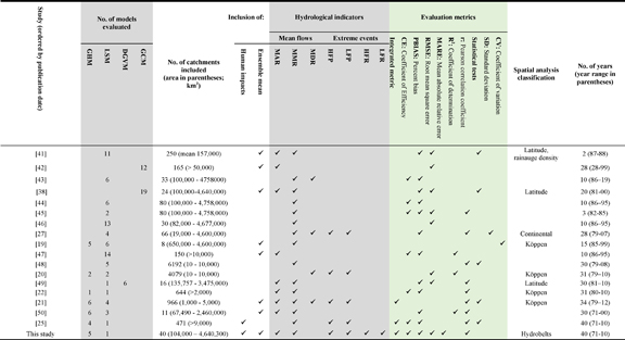 |
Firstly, only a handful of studies [19–22] have explored spatial patterns of model performance, all of them by using the Köppen climate classification system. Here, for the first time, we evaluate the performance of several global-scale hydrological models across hydrobelts [23] (figure 1 and table S2; tables and figures in the supplementary information available at stacks.iop.org/ERL/13/065015/mmedia, hereafter called SI, are denoted by an S in their numbering). This offers a more appropriate classification scheme for catchment hydrology than the Köppen system because it takes into account a greater number, and diversity of, hydro-geographical factors in defining the boundaries of the spatial units.
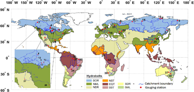
Figure 1. Locations of the 40 catchments across hydrobelts. Catchment details are provided in table S1. Hydrobelts are named: BOR= boreal, NML = northern mid-latitude, NDR = northern dry, NST = northern subtropical, EQT = equatorial, SML = southern mid-latitude, SDR = southern dry and SST = southern subtropical.
Download figure:
Standard image High-resolution imageSecondly, almost all previous evaluation studies compare simulations of naturalised discharge to observations. This means that the effects of human impacts on runoff and river flows remain unaccounted for by the models. This is despite the fact that the majority of catchments across the globe have been severely influenced by human activities [24, 25]. We capitalise on the latest model simulations conducted as part of the second phase of the Inter-Sectoral Impact Model Inter-comparison Project (ISIMIP2a), which provides a set of simulations that include time-varying human impacts, such as water abstractions and reservoir operations by dams [26]. In so doing and in parallel with a companion study presented in this journal issue [25], we conduct the first multi-model evaluation of runoff under human-impacted conditions as simulated by global-scale hydrological models.
Thirdly, with only a very limited number of exceptions [20, 21, 25, 27], it is uncommon for global-scale hydrological model evaluation studies to assess the ability of models to simulate hydrological extremes, particularly high and low runoff or specific return periods. We address this paucity of evidence by evaluating indicators of hydrological extremes, including specific return periods.
Fourthly, a multitude of different performance metrics have been employed within and between studies. The ranking of models, by performance, changes according to the metrics that are employed because different metrics emphasise different characteristics of model performance. To overcome this issue we use a novel integrated metric [28–31].
Finally, the ensemble mean (EM) is often used to summarise the performance of several models because it has been shown that the EM often performs better than the majority of the individual models from which it is derived [32–38]. However, not all studies have provided a comprehensive analysis of the performance of the EM relative to individual models, at global (table 1) and continental scales [39, 40]. Therefore, we evaluate the performance of six models individually, as well as the EM.
By capitalising on the five opportunities discussed above we provide a distinct contribution to understanding how global-scale hydrological models perform in different parts of the globe and for different hydrological indicators, including extremes.
2. Methods
2.1. Study catchments, models and data
2.1.1. Study catchments and observed data
Forty study catchments (figure 1 and table S1) were identified following a comprehensive set of four criteria (see SI) applied to observed data from the Global Runoff Data Centre, GRDC (available from http://grdc.bafg.de). The catchments provide a reasonable geographic coverage, however, the availability and quality of observed data in the GRDC database led to a selection bias that resulted in the number of boreal and northern mid-latitude catchments being proportionately high (table S2).
2.1.2. Model ensemble and forcing data
The model ensemble comprises a suite of GHMs and LSMs that participated in the water (global) sector of ISIMIP2a [51]. The models are DBH [52], H08 [53], LPJmL [54], MATSIRO [55], PCR-GLOBWB [56] and WaterGAP2 [57] (see SI for full model names and details of the hydrological processes represented in the models).
All of the models have been developed to represent and account for the impacts of historical time-varying human management such as land use, water use and dam operation. Apart from WaterGAP2 the models were not calibrated for the ISIMIP2a simulations. The models simulate runoff (amongst other hydrological variables) across the global land surface at 0.5° × 0.5° spatial resolution. Following the method described by [19], monthly observed and simulated discharge data was converted to catchment-mean monthly runoff by using the area upstream of the gauge according to the DDM30 river network. Thus an area correction factor is applied to the GRDC discharge data to account for the fact that the river network, which is at 0.5 ° spatial resolution, may not perfectly overlap with the GRDC river catchment boundaries. Output from the models is openly available from the Earth System Grid Federation (ESGF; https://esgf-data.dkrz.de; [51]).
All models were run for the period 1971–2010 with input climate data provided by the Global Soil Wetness Project Phase 3, (GSWP3; [58]). GSWP3 has been used as a forcing dataset in several other recent GHM and LSM studies [2, 26, 57, 59, 60] (see SI, section 1.3, for an explanation of why we used this forcing dataset specifically).
2.2. Evaluating model performance
2.2.1. The integrated evaluation metric
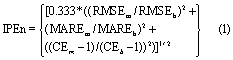
Assessment of relative model performance in a meaningful way is difficult without a transferrable benchmark against which model performance in different catchments can be compared to consistently. In addition, different metrics are more or less suited to assessing individual characteristics of a model's fit. To overcome this we use a ratiometric integrated metric, the ideal point error (IPE) [31], equation 1. Our configuration of IPE has three components because it combines three commonly used individual evaluation metrics: root mean square error (RMSE), Mean absolute relative error (MARE) and the Nash-Sutcliffe coefficient of efficiency (CE). These are used to assess the relative performance of each model and the EM to replicate observed data. IPE is standardised against a benchmarked model. The benchmark model can be a simple statistical model, so it is sometimes called a naïve model [61]. It can be as simple as observed runoff shifted backwards by different time steps [61]. In our application of IPE, we adopted a naïve model benchmark such as this, where the observed runoff is shifted backwards by one month. Hence our naïve model benchmark assumes runoff in month t is equal to runoff in month t−1 and therefore essentially assumes persistence (IPEn, equation 1). The three IPE components are evaluated against their benchmark model counterparts.
Table 2. Indicators of mean and extreme runoff calculated in this study for model evaluation.
| Indicator abbreviation | Description of indicator |
|---|---|
| MAR | Mean annual runoffa |
| MMR | Mean monthly runoffa |
| Q5 | The magnitude of monthly runoff that is exceeded 5 % of the time in the monthly time series (indicator of high flows)a |
| Q95 | The magnitude of monthly runoff that is exceeded 95 % of the time in the monthly time series (indicator of low flows)a |
| None | The magnitude of maximum monthly runoff associated with the 2-, 5-, 10-, 20-, and 25 year return periods respectively (see SI for calculation method)b |
| None | The magnitude of minimum 3 month moving average of runoff associated with the 2-, 5-, 10-, 20-, and 25 year return periods respectively (see SI for calculation method)b |
aFor these indicators the EM is calculated as a timeseries by calculating the average across all individual models for each month, to allow calculation of timeseries-based evaluation metrics such as the NSE and IPE. bFor the maximum and minimum return period flows the EM was calculated as the average of the maximum/minimum monthly runoff for each return period calculated across all GHMs.
The IPE equation presented in equation (1) is adapted from the original formula by (Dawson et al 2012). The negative reciprocal of the IPE score is used (equation 3) where the performance of a model exceeds that of the benchmark to maintain proportionality in comparisons between the IPE scores of models that fail to perform as well as the benchmark and those where performance exceeds it. The IPE scores range between −1 and −∞ (performance improvement over the benchmark model) and 1 and +∞ (performance loss over benchmark model). The IPE score is ratiometric—for example, a model that performs twice as well as the benchmark model will have an IPE score of −2 and a model that performs twice as badly will have a score of 2. IPE would be 1 if a model performs the same as the benchmark, whilst a model infinitely better than the benchmark would have an IPE of −∞.

If IPEn ≥1 i.e. where a model fails to outperform the benchmark model
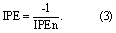
If IPEn <1 i.e. where a model outperforms the benchmark model
where:
RMSE = root mean squared error
MARE = mean absolute relative error
CE = coefficient of efficiency (Nash-Sutcliffe Efficiency)
m = model simulated data
b = benchmark (the naïve model).
2.2.2. Weighted performance measures and performance ranking
Where measures of performance are aggregated for an entire hydrobelt we do so by calculating a weighted mean, to resolve spatial biases introduced by having a different number of catchments in each hydrobelt. For each catchment, observed mean annual runoff (MAR), representing the effect of both catchment size and flow, is applied as the relative weight, so that any given weighted performance metric (Wm) can be calculated as:
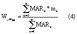
where m denotes metric, HB and c respectively denote hydrobelt and catchment, and n the number of catchments in each hydrobelt.
Measures of performance that we calculated and weighted in this way include IPE, percent bias (PBIAS) and the relative difference between simulated and observed values for the seasonal cycle (see table S4 for formulae). The median percentage difference (MPD) was calculated across all catchments but was not weighted.
For consistency throughout the paper, metrics derived for the EM are used to rank and/or facilitate comparisons between catchments or hydrobelts. This is not to say, however, that the EM is a reliable indicator of overall model performance.
2.2.3. Hydrological indicators
In addition to IPE and measures described in section 2.2.2 we calculated six indicators of mean and extreme runoff (table 2).
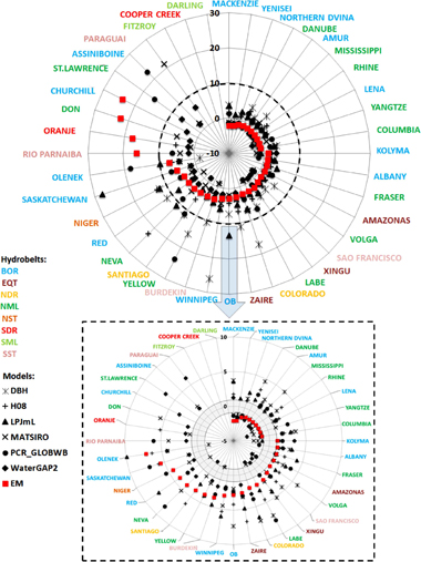
Figure 2. Catchments ranked clockwise (starting with Mackenzie) according to the IPE score for the ensemble mean (EM, red squares). IPE scores range between (−1, −∞] and [1, +∞). The bottom panel focuses on IPE≤10, with the range (−1,1) in grey, representing the boundary of performance improvements (IPE ≤ −1) or loss (IPE ≥ 1) relative to the naïve benchmark model. Catchment names are colored by hydrobelts (BOR = boreal, NML = northern mid-latitude, NDR = northern dry, NST = northern subtropical, EQT = equatorial, SML = southern mid-latitude, SDR = southern dry and SST = southern subtropical).
Download figure:
Standard image High-resolution imageTable 3. Mean weighted IPE for each model by hydrobelt. Negative (positive) values indicate performance improvement (loss) over the naïve model benchmark. Best performing individual models for each hydrobelt are in bold. Number of catchments in each hydrobelt are in parentheses. Hydrobelts are ranked according to the perfomance of the EM. Rows are ordered according to the mean latitude of each hydrobelt from north to south (BOR = boreal, NML = northern mid-latitude, NDR = northern dry, NST = northern subtropical, EQT = equatorial, SML = southern mid-latitude, SDR = southern dry and SST = southern subtropical).
| Model | |||||||||
|---|---|---|---|---|---|---|---|---|---|
| Hydrobelt (No. of catchments) | DBH | H08 | LPJmL | MATSIRO | PCR-GLOBWB | WaterGAP2 | EM | Hydrobelt rank (based on EM) | Hydrobelt rank (based on best individual model) |
| BOR (14) | 25.63 | 5.33 | 8.12 | 2.52 | 3.53 | 1.12 | 2.07 | 2 | 5 |
| NML (12) | 53.08 | 12.76 | 9.87 | 7.20 | 5.87 | −0.30 | 3.90 | 4 | 1 |
| NDR (2) | 14.53 | 4.09 | 4.71 | 4.32 | 7.46 | 0.95 | 2.96 | 3 | 3 |
| NST (1) | 12.10 | 12.89 | 12.10 | 1.82 | 5.39 | 1.12 | 4.32 | 5 | 4 |
| EQT (3) | 4.82 | 3.28 | 3.65 | 1.93 | 2.95 | 0.57 | 1.67 | 1 | 2 |
| SST (4) | 26.91 | 21.86 | 19.53 | 2.55 | 13.40 | 1.38 | 10.58 | 6 | 6 |
| SDR (2) | 5305.19 | 96.43 | 2051.53 | 326.04 | 520.61 | 78.19 | 1393.72 | 8 | 8 |
| SML (2) | 2780.76 | 109.56 | 1440.15 | 128.58 | 958.59 | 42.15 | 909.93 | 7 | 7 |
| Median weighted IPE across all hydrobelts | 26.27 | 12.82 | 10.99 | 3.44 | 6.67 | 1.12 | 4.11 | — | — |
| Model rank (based on median weighted IPE across all hydrobelts) | 6 | 5 | 4 | 2 | 3 | 1 | |||
3. Results
3.1. Models' ability to replicate observed monthly runoff time series
IPE scores estimated from the monthly runoff timeseries for individual models and the EM respectively, across hydrobelts, are presented in figure 2 (see table S6 for individual catchments and figure S1 for the individual metrics that comprise the IPE). Model performance is generally better in the equatorial and northern hydrobelts (EQT, BOR, NML, NDR and NST) than the southern hydrobelts (SST, SDR and SML). When ranked by the EM, the 13 highest ranked catchments are located in BOR and NML hydrobelts. This is in part the result of a bias in the number of catchments in these hydrobelts. However, weighted IPE scores (table 3) indicate that model performance in these two hydrobelts is particularly favourable when compared to that of southern hemisphere hydrobelts. The two SML catchments are ranked 38th and 40th and the two SDR catchments are ranked 32nd and 39th. The relatively lower performance of the majority of models and the EM in the SDR and SML hydrobelts, which include seasonally dry ephemeral rivers, is the result of the models slightly overestimating low runoff values (typically less than 1 mm month−1) during dry periods. This serves to decrease the MARE (figure S1), which in turn delivers poor IPE values. We considered lowering the weighting of the MARE component of the IPE equation, since the three components can be weighted differently [31] so that the IPE is not disproportionally affected by the low MARE scores in these four catchments. However, this would be somewhat counter-intuitive to the objectives of our assessment because the low MARE values highlight that the models struggle to simulate low flows in these catchments, which is an important result of the evaluation exercise.
The EM and all individual models except WaterGAP2 and marginally MATSIRO, deliver their best IPE in the EQT hydrobelt. Here, the three contributing catchments cover 51% of its area; indicating that they are representative of the hydrobelt as a whole. However, the strong model performance is, in part, an artefact of using the naïve (t−1) model as a benchmark for computing IPE scores. In EQT catchments the month-to-month variability of hydrological inputs and responses is low, which makes the modelling challenge easier and the likelihood of significant deviation from the naïve benchmark model relatively low.
Download figure:
Standard image High-resolution image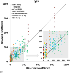
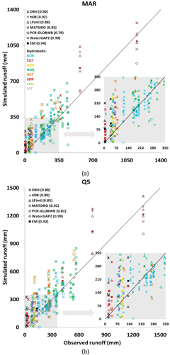
Figure 3. Simulated versus observed MAR (a); Q5 (b); and Q95, (c) for each catchment (n = 40). The numbers in parentheses indicate the Pearson correlation coefficients between simulated and observed data (BOR = boreal, NML = northern mid-latitude, NDR = northern dry, NST = northern subtropical, EQT = equatorial, SML = southern mid-latitude, SDR = southern dry and SST= southern subtropical).
Download figure:
Standard image High-resolution imageExamining the performance of individual models, it is evident that H08 performs relatively well (second to WaterGAP2) in the NDR hydrobelt as well as the two lowest ranked hydrobelts i.e. SDR and SML, suggesting it has particular capabilities in modelling dry regions. The calibrated WaterGAP2 outperforms the EM and other models in all hydrobelts, however, it is not always the best performing individual model. Indeed, MATSIRO achieves the best IPE scores in six catchments (table S6). In terms of the IPE, the EM performs better than the best model only in two catchments, the Amur and Mackenzie—for the other 38 catchments an individual model performs better than the EM.
To further investigate the performance of the EM, we calculated the EM under two different cases:
- 1.excluding the weakest performing model for each catchment in turn; and
- 2.excluding the first and second weakest models for each catchment in turn.
The best/weakest models that were left in the ensemble were identified based on the models' IPE scores.
Under the two cases, the EM outperformed the best individual model that was left in the ensemble in ten and 12 catchments respectively (table S6). Thus the relative performance of the EM, compared to the models that are left in the ensemble, improves when the weakest performing model(s) are removed. However, in the majority of catchments, even when the weakest performing model(s) are removed from the ensemble, an individual model still performs better than the EM.
3.2. Models' ability to reproduce key aggregated hydrological indicators
The PBIAS and MPD across catchments indicate a general trend towards the over-estimation of mean annual runoff (MAR), Q5 (high runoff) and Q95 (low runoff) amongst the models, especially for low(er) runoff values (figure 3, table 4 and table 5). In terms of individual model performance, WaterGAP2 and MATSIRO are ranked first or second by both MPD (table 4) and PBIAS (table 5) for all three indicators, whereas DBH is consistently ranked the lowest.
In terms of model performance across hydrobelts, the three best estimates of weighted PBIAS for all three hydrological indicators are, according to the performance of the EM, consistently BOR, NML and EQT, (table 5). The EQT hydrobelt is consistently highly ranked (top 3) according to the performance of both the EM and the best performing individual model, whilst the SML and SDR hydrobelts are always ranked low. The ranking of hydrobelts changes slightly when evaluating performance with MPD (table S5). Although BOR and NML are still ranked highly (top 3 for all three hydrological indicators) EQT is lower down the ranking (ranked 6th for all three hydrological indicators).
3.3. Models' ability to estimate runoff of different return periods
Table 6 presents the MPD between modelled and observed runoff calculated over all catchments for each of the five return periods (2-, 5-, 10-, 20- and 25-year) of maximum monthly runoff and minimum 3 month runoff respectively. For maximum runoff, PCR-GLOBWB performs particularly well, with MATSIRO and WaterGAP2 also delivering MPD values of <25%. The remaining models perform relatively poorly with the MPD >50% across all return periods. For minimum runoff, MATSIRO again performs well, with DBH also achieving MPD values of <20%. Despite being calibrated, WaterGAP2 (and PCR-GLOBWB) struggles to reproduce observed low runoff, with MPD values generally >50%.
The magnitude of runoff associated with each return period for both maximum and minimum runoff is overestimated by the EM and by the majority of individual models. The EM fails to perform better than the best performing model for all maximum and minimum flow return periods. In half of all cases, MPD values are generally consistent across the different return periods, while MPD decreases or increases with higher return periods in other cases.
3.4. Models' ability to replicate seasonal cycles
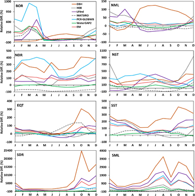
Figure 4 displays for each hydrobelt the average weighted relative difference (using equation 4) between the modelled and observed seasonal cycle (long-term MMR) for all models. There is a general pattern of overestimation of MMR across the model ensemble. The largest relative differences occur in the months of peak runoff. No single model performs consistently better or worse than all other models throughout the whole seasonal cycle, since the month in which the maximum relative difference occurs varies across models.
The highest magnitude differences are observed in the SDR and SML hydrobelts. The lowest are in NML and EQT. The models' poor performance in simulating long-term MMR in the SDR hydrobelt confirms their poor performance in replicating the time series of runoff in this hydrobelt (table 3). This suggests that timing errors may be responsible for much of the error in simulating runoff timeseries in the SDR hydrobelt.
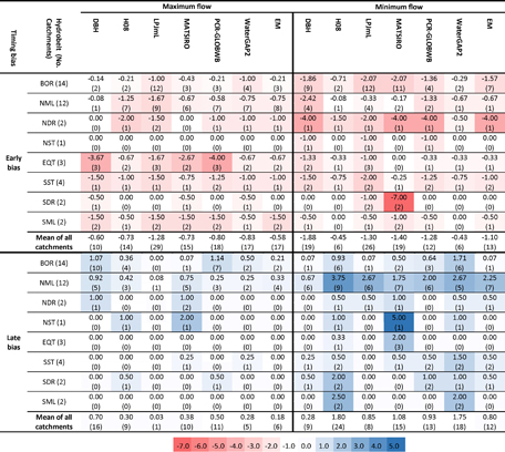
Table 7 shows the duration, in months, of the difference between simulated and observed timing of the month of maximum/minimum runoff, i.e. timing bias, as an average for each hydrobelt (figure S2 displays the simulated and observed MMR for each catchment). Early bias is common in all hydrobelts and it is especially prevalent for minimum flows. Late bias is less evident. Two potential explanations for early bias are the models' inability to capture late snowmelt in snow-dominant regions [62] and challenges in accurately representing groundwater or baseflow [55].
Across all models and catchments, DBH shows the least early (−0.60 months) and LPJmL the least late (0.03 months) biases for maximum flow. For minimum flow, WaterGAP2 presents the least early bias (−0.43 months) and DBH shows the least late bias (0.28 months). Despite the good performance of DBH and LPJmL in terms of timing, these two models do show high relative difference values compared to other models (figure 4).
Table 4. Median percentage difference, MPD (%) between modelled and observed runoff calculated over all catchments for MAR, Q5 and Q95 (shaded cells denote underestimation of runoff by the model; ranking of the individual models across each indicator are in parantheses). The best performing individual model (or EM) is in bold.
| Indicator | DBH | H08 | LPJmL | MATSIRO | PCR-GLOBWB | WaterGAP2 | EM |
|---|---|---|---|---|---|---|---|
| MAR | 33.7 (6) | 20.1 (5) | 13.5 (4) | −12.6 (3) | 7.8 (2) | 0.9 (1) | 13.9 |
| Q5 | 26.2 (6) | 15.3 (5) | 12.2 (4) | −11.8 (3) | 5.1 (2) | −2.9 (1) | 9.6 |
| Q95 | 37.3 (6) | 19.4 (5) | 19.1 (4) | −8.8 (2) | 14.6 (3) | 5.0 (1) | 21.0 |
Table 5. Mean weighted PBIAS (%) for MAR, Q5 and Q95, across hydrobelts. The best performing model (or EM) according to weighted PBIAS for each hydrobelt is in bold. Shaded cells denote where the runoff indiciator is underestimated by the model or EM. Hydrobelts are ranked according to the perfomance of the EM. Rows are ordered according to the mean latitude of each hydrobelt from north to south (BOR= boreal, NML= northern mid-latitude, NDR= northern dry, NST = northern subtropical, EQT = equatorial, SML= southern mid-latitude, SDR= southern dry and SST= southern subtropical).
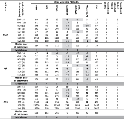 |
Table 6. Median percentage difference, MPD (%) between modelled and observed runoff calculated over all catchments for different return periods (shaded cells denote underestimation of runoff by the model). The best performing model (or EM) is in bold.
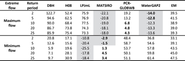 |
Table 7. Hydrobelt mean (not weighted) early and late runoff timing bias (units are number of months). Negative (positive) values denote an early (late) bias. Values calculated over all catchments across each hydrobelt, or globally. The number of catchments affected by timing bias is in parantheses. Rows are ordered according to the mean latitude of each hydrobelt from north to south (BOR = boreal, NML = northern mid-latitude, NDR = northern dry, NST = northern subtropical, EQT = equatorial, SML = southern mid-latitude, SDR = southern dry and SST = southern subtropical).
 |
4. Discussion
4.1. Models' performance across hydrobelts
We found high variability between models in their ability to simulate MAR, Q5, Q95 and the magnitude of return period runoff values. The majority of models overestimate these hydrological indicators, with positive biases particularly acute in southern hydrobelts (SML and SDR). This can, in part, be explained by the general overestimation of precipitation values in climate forcing data in these regions [57], which in turn means the models overestimate runoff [21]. Nonetheless, previous studies emphasise that large ensemble spreads from GHMs and LSMs are not primarily due to errors in the (common) forcing data, but instead due to model structural uncertainty [19, 39]. Missing physical process representations in the models such as transmission loss [62] explain some of the differences between simulated and observed runoff. The underestimation of runoff by certain models, particularly in the NDR hydrobelt, may be a result of excessive evapotranspiration (as reported for MATSIRO by [19]). Moreover, the simulation of evapotranspiration has been shown to vary widely between the ISIMIP2a global-scale hydrological models [63].
Several models struggle to accurately simulate the timing and magnitude of long-term MMR in all months of the year in NDR and the first and/or last months in other hydrobelts. The relatively low levels of season-to-season variability in tropical and equatorial catchments EQT, SST and NST (i.e. the absence of a strong, predictable signal that can be modelled) may explain the weak performance in these hydrobelts. Additional factors may include the ability of models to sufficiently represent the range of soil properties influencing the generation and timing of runoff [64], as well as human-induced factors such as the operation of different reservoir management schemes [25]. In the BOR hydrobelt, the simulation and representation of snowmelt is likely to be the main cause of the early bias we reported. Temporal bias in snow-dominant regions (observed in [20, 21, 27, 40, 43, 65]) has previously been related to general errors in forcing data (especially the underestimation of precipitation) or the absence/misrepresentation of processes that delay snowmelt in models. Some of these processes include the infiltration of meltwater into soils, the refreezing of meltwater over cold periods in the diurnal cycle, and ice-jams in rivers [21].
Figure 4. Mean weighted relative difference between simulated and observed MMR (seasonal cycle) for each hydrobelt (note that vertical scales differ) (BOR = boreal, NML = northern mid-latitude, NDR = northern dry, NST = northern subtropical, EQT = equatorial, SML = southern mid-latitude, SDR = southern dry and SST = southern subtropical).
Download figure:
Standard image High-resolution image
The higher timing bias we found for minimum runoff is related to the observed data's higher sensitivity to the timing of water abstractions and reservoir operation during low flow periods [25]. Nonetheless, it should be emphasised that the degree to which monthly flow is influenced by reservoirs depends on the ratio of reservoir storage and the annual flow. With large reservoirs, any model's ability to simulate storage and release of water can be more important than, for example, the timing of snowmelt.
Whilst when aggregating across catchments WaterGAP2 is consistently the best performing model in terms of overall fit (assessed by mean weighted IPE, table 3), consistently the best for MAR, Q5 and Q95 when assessed by MPD (table 4), and almost always the best model for MAR, Q5 and Q95 when assessed by mean weighted PBIAS (table 5), it is not the best model for the magnitude of flows associated with different return periods (table 6) nor for the timing of seasonal flows (table 7). For these latter two hydrological indicators, the best performing models include MATSIRO, H08 and PCR-GLOBWB. This is in part due to the global-scale models having spatially generalised parameters. Thus they may perform differently in different locations and for different indicators. In addition, although they all use the same forcing data, differences in model structure and parameterisation (table S3) lead to different performances across different indicators [64, 66, 67]. Thus caution should be applied in presenting the results from only one model (including the ensemble mean) in future model applications, where changes in multiple hydrological indicators are presented. Instead, we recommend the ensemble spread is presented and/or models are weighted according to their performance for each hydrological indicator respectively [68].
Generally, the superior performance of WaterGAP2 can be attributed to its calibration with long term annual average river discharge. However, our results show that this approach does not necessarily guarantee optimal performance for all hydrological indicators, e.g. high and low flows. Moreover, due to limitations associated with the quality, length and global coverage of observed discharge data, WaterGAP2 was only calibrated for 1319 catchments, covering 54% of the global land area except Antarctica and Greenland [57]. Thus the model is unlikely to achieve optimal performance globally, for all hydrological indicators. The physically-based snow and soil scheme in MATSIRO may be the reason for its superior performance in snow-dominated areas. DBH and PCR-GLOBWB presented higher skill in simulating maximum runoff of higher return periods. DBH also achieved good performance in simulating the timing of the seasonal cycle.
4.2. Opportunities for model improvement
WaterGAP2, the only calibrated model in the ensemble, presents the greatest overall model skill. However, WaterGAP2 is not the best-performing model (with respect to IPE) in 13 of the 40 catchments—ten of these are in the BOR hydrobelt. The result arises from the calibration of WaterGAP2 to match observed long-term annual river discharge, meaning that the model is prone to timing errors in snow dominant regions [69]. Conversely, the superior, physically-based snow and soil scheme in (uncalibrated) MATSIRO is likely to be a key reason for its good performance in snow-dominated hydrobelts. That said, H08 uses a similar snow modelling scheme to MATSIRO and does not attain a similar level of performance in the BOR hydrobelt. This suggests that H08's vegetation, evapotranspiration and soil representation schemes (all of which are different to MATSIRO) may be limiting its performance.
Our results imply that robust calibration methods may improve model performance. However, a smaller error in runoff estimates for a present-day hydrological simulation (from an uncalibrated or calibrated model) does not necessarily mean that projections for the future from that model will be more certain than projections from a model with larger error. Whilst the calibration procedure for WaterGAP2 does lead to better performance for present-day hydrology in many cases, we note that the calibration of any hydrological model can encourage over-fitting and so act to compensate for structural errors and errors in atmospheric forcing data [69]. This could pose a problem if the models were used within a climate modelling framework. Therefore, whilst this study highlights the benefits of model calibration for improving simulations of present-day runoff, we also urge caution towards interpreting it as a definitive route to higher model certainty; especially when the models are used for delivering future projections [70].
DBH and PCR-GLOBWB were able to achieve a reduction in the magnitude of error in simulated maximum runoff with increasing return period. It was more common for the other models to show little difference in error across return periods. This suggests that these two models may include process representations that work better towards achieving very extreme high flows, compared with other models.
Our results show that even when including human impacts, there remain challenges with the accurate simulation of low runoff magnitudes and long term MMR. Therefore we recommend a comprehensive and systematic evaluation of the specific methods used to represent human impacts in models, for multiple rivers across the globe and at different locations along the river network, including: irrigation; dam operation rules [26]; the representation of reservoirs; the way in which withdrawn water is returned to the river network (including groundwater, surface water bodies and soils); and the sources where water is withdrawn from to meet water needs (i.e. groundwater, surface water, and desalinisation).
4.3. Performance of the EM and implications for future applications
In climate modelling and meteorological forecasting, the ensemble mean is often reported as outperforming individual models [34–36]. Our analysis shows that this is not the case with global-scale hydrological models. Even when excluding the weakest performing model(s) from the ensemble an individual model still outperforms the EM in the majority of catchments. We only excluded up to two weakest performing models when computing the EM under different cases, so the generally consistent weak performance of the EM may be the result of other outlying models (in terms of their performance) having a large disproportionate influence on the EM.
Certain models may be consistently poor performers in certain climatic or physiographic settings, or over certain hydrological response ranges, and their inclusion in a model ensemble may act to limit the performance of the EM [71]. However, totally excluding the weakest model might be at the risk of missing other skills of that model. For example, whilst DBH performed poorly for some hydrological indicators, it performed well in simulating timing of the seasonal cycle. The approach of including/excluding the best/weakest performing models to calculate the EM could be extended to weighting methods [68, 72–74]. This, however, raises difficult questions about how the 'best' weighting strategy and combination of weights can be determined a priori.
The variable performance of the EM that we report here means that a decision should not be taken a priori to use the EM as the basis of model evaluation and/or climate change impact assessments [1, 21, 39, 75] without considering its performance relative to the models it is summarising, because an individual model may perform significantly better.
5. Conclusion and recommendations
We have presented a worldwide comparative evaluation of the performance of six global-scale hydrological models to simulate mean and extreme monthly runoff. In parallel with a companion study presented in this journal issue [25], it is the first such evaluation to use models run with human impacts and it is also the most comprehensive evaluation of extreme runoff (table 1). Our adoption of the hydrobelt classification system provided a feasible means of aggregating catchment-scale results around the axis of hydro-geographical similarities, as well as facilitating a comparison of model performance spatially worldwide.
We found a tendency for the majority of models to overestimate MAR and all indicators of upper and lower extreme runoff. The models overestimate low flows (Q95) considerably more than they overestimate high flows (Q5) but on the other hand, the models overestimate minimum flow return periods to a lesser degree than they do for maximum flows. Either way, the overestimation of runoff is a key issue that we recommend is addressed by the global-scale hydrological modelling community. Whilst the incorporation of human activities into global-scale hydrological models has been shown to enhance model simulation capabilities [25], our evaluation leads us to recommend that the global-scale hydrological modelling community pursue efforts to improve the representation of low runoff and the models' ability to predict the magnitude and timing of seasonal cycles.
We have highlighted which models perform particularly well for certain hydrological indicators, and in which hydrobelts, and discussed potential solutions to improving model performance. Whilst calibration can deliver some improvements it is particularly challenging for global-scale models due to the paucity of global coverage of long-term and complete observed runoff records. Therefore we recommend that efforts are made towards improving the quality [76, 77] and global coverage of observed runoff records and in turn technical approaches to model calibration are explored.
Other model improvements can be achieved through better quality input and evaluation datasets, the inclusion of missing physical processes, and better representation of existing processes in the models. We recommend that the global-scale hydrological modelling community explore the process parametrisations within their models to help inform their decisions on future model development and that they consider running perturbed parameter ensembles [78] to explore the uncertainties associated with those parametrisations.
While the EM is a straightforward, widely used means of summarising the performance of an ensemble of hydrological models, our results highlight the limitations of this approach. Therefore we recommend the exploration of alternatives to the EM such as weighting models based upon their performance [68]. Nevertheless, the models that comprise the ensemble we evaluated here, represent the state-of-the-art, and multi-model ensembles may well be the best way to capture some of the existing uncertainties in representing the hydrological cycle at the global scale. Therefore we recommend that future studies adopt an ensemble approach so that the spread of possible outcomes, based upon current scientific modelling state-of-the-art, is known. The value of ensembles lie in their offering of a suite of models that can be evaluated with respect to a specific question that might need addressing. For example, if droughts were of interest, then one may possibly select a subset of models that is different from a subset that might be used if peak flows were of interest. Such a procedure can of course only be undertaken if the full range of model simulations are available in the first place.
The models evaluated here are under continuous development and we expect that their performance will improve as developers address known shortcomings and as observed data improves in quality. Model improvements will then in turn lead to more precise and accurate representation of hydrological patterns across the globe.
Acknowledgments
This work has been conducted under the framework of the Inter-Sectoral Impact Model Intercomparison Project, phase 2a (ISIMIP2a), so our thanks go to the modellers who submitted results to this project. The ISIMIP2a was funded by the German Ministry of Education and Research, with project funding reference number 01LS1201A. Data is available from [51]. We also thank the Global Runoff Data Centre (GRDC) for making available the observed runoff data. JZ was supported by the Islamic Development Bank and a 2018 University of Nottingham Faculty of Social Sciences Research Outputs Award. IH was supported by grant no. 243803/E10 from the Norwegian Research Council. JS was supported within the framework of the Leibniz Competition (SAW-2013 PIK-5) and by the EU FP7 HELIX project (grant no. 603864). JL was supported by the National Natural Science Foundation of China (41625001, 41571022), the Beijing Natural Science Foundation Grant (8151002), and the Southern University of Science and Technology (Grant no. G01296001). GL was supported by the Office of Science of the US Department of Energy as part of the Integrated Assessment Research Program. PNNL is operated by Battelle Memorial Institute for the US DOE under contract DE-AC05-76RLO1830. NH and YM were supported by the Environment Research and Technology Development Fund (S-10) of the Ministry of the Environment, Japan. HK and TK were supported by Japan Society for the Promotion of Science KAKENHI (16H06291).