Abstract
Lithium-ion batteries are typically charged using constant current that is applied until the cell voltage reaches about  , at which time, charging continues at a constant voltage until the full battery capacity is attained. This process is slow, typically requiring
  . Empirically selected pulse-charging sequences have been shown to provide enhanced charging; however, no model exists to explain and optimize the pulse-charging protocols. Modeling the lithium diffusion into a homogeneous intercalant layer indicates that the lithium concentration reaches saturation at the graphite∕electrolyte interface after about
  under conventional constant current charging, mandating the shift to the lower rate constant voltage charging. It is shown here that charging the lithium battery using non-dc waveforms with properly selected parameters may circumvent this lithium saturation, enabling charging at significantly higher rates. A nonlinearly decreasing current density profile which conforms to the mass transfer coefficient variation was shown to provide complete charging in less than
  of an hour, faster than any other pulse-charging profile studied.
Export citation and abstract BibTeX RIS
Lithium is particularly advantageous as the negative electrode material in batteries because of its very negative standard potential  , low specific gravity, and wide availability. However, lithium metal cannot be safely used in rechargeable batteries because of dendritic deposition,1 which may lead to shorting and as a consequence to thermal runaway.2 Furthermore, the highly active lithium reacts with the electrolyte. Nonlevel deposition accompanied by reaction with the electrolyte often leads to electrically isolated regions containing the active material (lithium) resulting in lower capacity. To overcome this, lithium is being intercalated into a carbon or graphite matrix on the negative electrode,3 still maintaining a high voltage (
 vs
vs  ), high capacity (
 of graphite mass), and high energy density
  .
.
Conventional lithium-ion battery charging is typically done in two stages, as shown in Fig. 1. The battery is first charged at a constant current until the cell voltage reaches the upper voltage limit of  . This is followed by a second, constant voltage charging stage until the current drops to about 3% of its rated value. The charging time for the first stage (constant current) is typically
  , during which time about 88% of the battery capacity is charged. The second stage (constant voltage) takes about
  , extending significantly the charging time of the battery.4 Charging the battery at higher voltages (i.e., exceeding
  ) or at higher current densities typically leads to decreased cycle life5 and rapid buildup of internal resistance, probably due to excessive buildup of the film forming at the solid electrolyte interface (SEI).6–9 The underlying reason for these phenomena is the formation of metallic lithium at the electrode-electrolyte interface. This buildup is due to imbalance between the lithium formation rate, which is proportional to the (charging) current density, and the diffusion rate of the formed lithium into the graphite.

Figure 1. Schematic of the conventional charging characteristics of the lithium battery. During the initial stage ("1"), charging is at a constant current density of about  as shown in (A), while the voltage is rising (B).
  designates the transition time at which the voltage reaches a value of about
  and the charging mode is switched to stage 2, where charging continues at a constant voltage while the current is continuously decreasing. As shown in (C), about 88% of the capacity is charged in stage 1 while the remaining capacity (about 12%), is charged in stage 2.
Pulse charging of lithium-ion batteries4, 10, 11 with relaxation periods occasionally accompanied by short discharge pulses has been shown empirically to result in faster charging. However, no adequate explanation as to why pulse charging is more effective in providing higher charging rates (as compared to conventional charging) has been offered. In this study, lithium diffusion into the graphite intercalant layer is modeled under both conventional charging and current pulsing. During charging, lithium ions diffuse through the electrolyte and are reduced at the graphite∕SEI interface, as shown schematically in Fig. 2 and 3. The reduced lithium diffuses into the graphite and intercalates. However, if the current density is too high, the lithium formation by reduction at the electrode interface exceeds the rate at which it can intercalate, and metallic lithium will start accumulating at the interface, negating the critical function of the intercalant. This lithium accumulation at the interface limits the maximum rate at which the battery can be charged. We present here a model based on a macrohomogeneous analysis of lithium diffusion into the intercalant for both conventional and pulse charging. We show that, by proper selection of the current waveform parameters, the capacity range over which lithium does not saturate at the interface can be extended, thereby significantly enhancing the charging rate.
Theoretical Model
Description of the lithium cell
A schematic representation of the lithium-ion cell is shown in Fig. 2. The negative electrode consists of a porous graphite layer connected to a copper current collector, and the positive electrode consists of cobalt oxide in contact with an aluminum current collector. A separator impregnated with a liquid electrolyte solution containing lithium ions or a polymer electrolyte film separates the electrodes. During the charging process, intercalated lithium is electrochemically oxidized at the cobalt oxide positive electrode to form lithium ions

Simultaneously, lithium ions are electrochemically reduced and intercalated into the graphite electrode matrix

The values of  and
and  depend on the structure of the intercalant and the state of charge. Typical values for
  and
and  range from about 0.2 to 0.95 and 0 to 0.94, respectively.
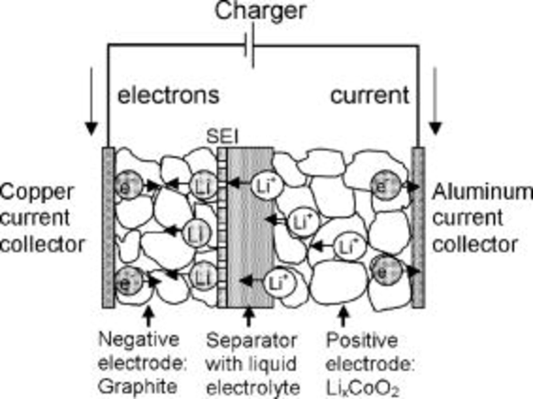
Figure 2. Schematic representation of mass and charge transport in a lithium-ion battery during charging.
During the first charging cycle, the solution species next to the graphite electrode are reduced at about  vs
vs  to form a film, the solid electrolyte interface (SEI).6, 12 This film effectively passivates the lithium intercalation electrode, allowing only lithium-ion migration while preventing insertion of electrolyte into the graphite.13–16
Two distinct lithium diffusion zones at the negative electrode
As shown in Fig. 3, two separate regions, where concentration polarization may arise, can be identified near the negative electrode (graphite). Only the left half of the cell corresponding to the negative graphite electrode is of interest to this analysis because lithium diffusion in graphite is slower than in the positive cobalt oxide.17–20 Hence, our analysis will focus on the lithium-ion reduction during charging and the subsequent lithium diffusion into the graphite, which is considered to be the limiting process. However, the principles and the analysis provided here can be similarly applied to lithium battery systems that are limited by lithium diffusion in the positive electrodes (cobalt oxide). Concentration polarization occurs in the electrolyte because of lithium-ion diffusion due to the charging current (right side, Fig. 3). Another source for concentration polarization is the slow diffusion of lithium within the graphite (left side, Fig. 3). This lithium is formed by the reduction of the lithium ions at the graphite-SEI interface, as indicated schematically in Fig. 3.
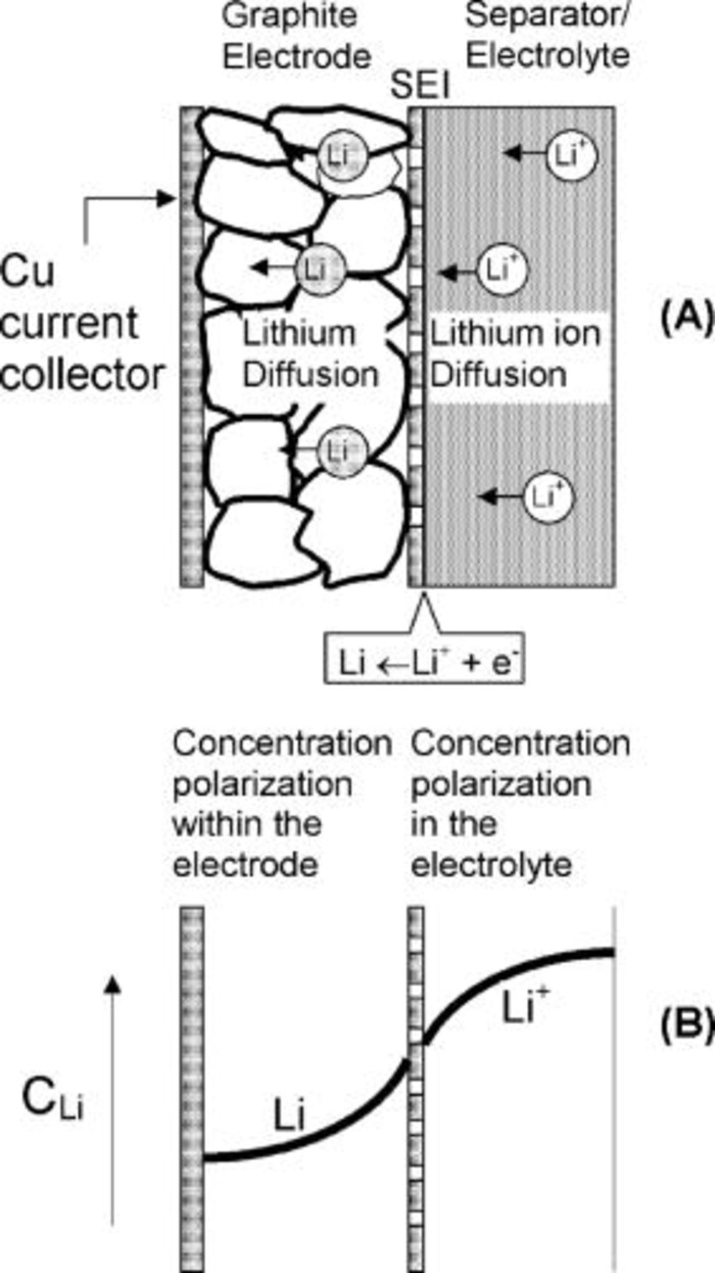
Figure 3. Lithium transport and concentration gradients at the negative electrode. (A) A schematic diagram (cross section) through the Li electrode and the electrolyte adjacent to it. (B) Two distinct concentration gradients, one in the electrolyte and the other within the graphite electrode, are schematically depicted. Lithium ions diffuse towards the cathode (on the left) and are reduced at the graphite∕SEI interface. The metallic lithium diffuses then into the intercalant on the left.
Lithium diffusion within the graphite
The graphite matrix is assumed to be homogeneous. It is further assumed that all lithium-ion reduction occurs at the graphite∕SEI interface and no reaction occurs within the graphite matrix. The intercalant typically is made of a complex structure consisting of channels, layers, or spheres. However, for modeling the macroscopic transport effects we do not take into account the internal structure of the intercalant and instead consider a homogeneous layer with an average or equivalent diffusion coefficient. This approach is similar to that involved in the classical macrohomogeneous modeling of porous electrodes.21 Figure 4 shows a schematic of the concentration profiles of lithium diffusing from the SEI into the graphite. The equation governing the lithium diffusion is
Here,  is the diffusion coefficient of lithium within the graphite. It is assumed to be a constant.
  is expected to actually depend on the degree of intercalation. However, literature data for this dependence are inconsistent. To simplify our model, we assume a constant value for
  that can be viewed as an integrated average. The effect of variations in the value of
  is discussed later on. The positive-
 direction points from the interface toward the graphite interior. The initial condition and the boundary conditions are given by Eq. 4, 5, 6. We assume that the lithium concentration within the graphite before charging starts is zero. Therefore, the initial condition is

The diffusion flux at the boundary,  (graphite∕SEI interface), is given by the applied current density
The flux at the outer intercalant boundary (the copper current collector, Fig. 4) at  is zero, as lithium cannot diffuse further
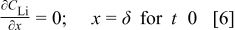
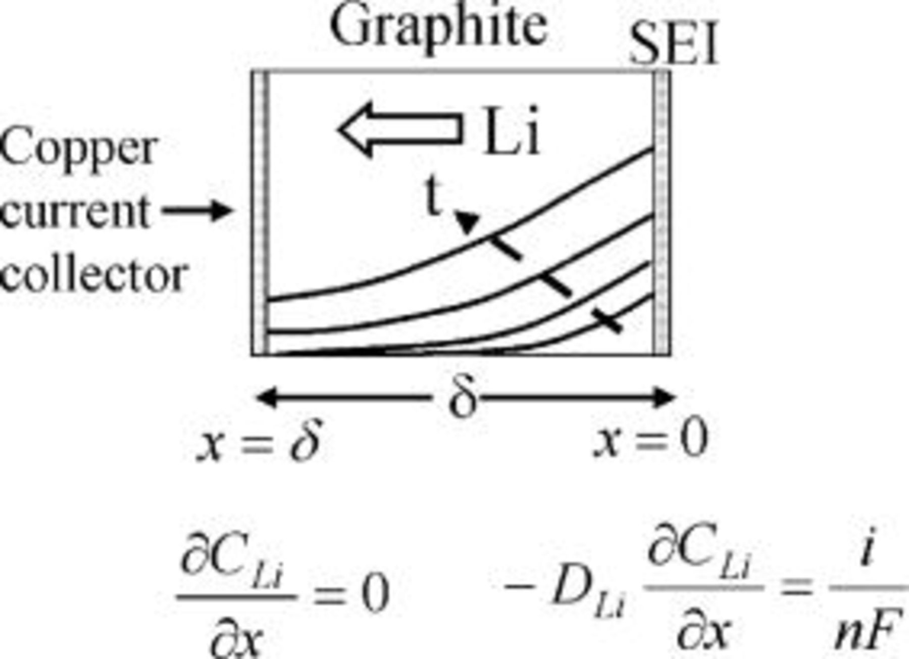
Figure 4. Schematic representation of the lithium diffusion from the SEI into the graphite. Time- and position-dependent concentration profiles are shown schematically.
Solution for the constant current case
The diffusion equation along with its initial and boundary conditions was solved using separation of variables.22, 23 The lithium concentration as a function of time,  , and distance from the graphite∕SEI interface,
  , is
, is

where  is the number of eigenterms.
Solution for the pulsed current case
Pulsed current was modeled by solving Eq. 3 subject to the initial and boundary conditions, Eq. 4, 5, 6. In Eq. 5, however, the current density was stepped to the specified values as the current pulse was applied. The solution was obtained by applying the superposition principle to Eq. 5. Rosebrugh and Miller24 used the superposition principle in their classical paper investigating the changes in concentration brought about by diffusion for a variety of periodic current waveforms. We have applied this principle to nonperiodic current waveforms.23 To illustrate the superposition principle, consider any two-pulse sequence. This sequence can be obtained by adding two constant current steps of different magnitudes and polarity starting at different times. The solution to the two-pulse sequence is obtained by adding the solutions of the two different current steps. Any multiple-pulse sequence can be similarly modeled. More details are provided in an earlier publication.23
Simulation and Discussion of Conventional Charging
Limitation of conventional charging
If the rate of lithium formation at the graphite∕SEI interface, which is controlled by the current density,  , is higher than the rate of lithium diffusion into the graphite,
  , lithium will accumulate at the negative electrode∕electrolyte interface during charging. This will eventually nullify the function of the graphite intercalant and expose the battery to potential dendritic growth, decreasing capacity and runaway situations. Therefore, charging of the lithium battery must be conducted such that no metallic lithium accumulates. This condition imposes a limit on the conventional charging rate during stage 1, where constant current charging is applied (Fig. 1). Furthermore, the transition to the constant voltage-charging mode (stage 2), during which the current density rapidly drops, becomes necessary due to the inability of the lithium to diffuse away at a sufficiently high rate. In the model, we assume that mass transport effects, rather than kinetics, control the lithium charging process. This assumption is consistent with the observation that there is a finite limit to the practical charging rates and that the time constants associated with the charge and discharge processes are similar to those expected for lithium diffusion through intercalant layers.
Simulations of conventional charging rates as a function of time, capped by the lithium concentration at the graphite∕SEI interface approaching the saturation level (just prior to the formation of metallic lithium), were modeled. A graphite electrode thickness of  , in accordance with the literature,20, 25 was considered throughout this work. We assume here that the limit on the charging process is when the concentration of the metallic lithium (within the graphite) reaches the saturation level of
  . In reality, harmful effects due to excessive lithium concentration may occur prior to lithium reaching its saturation level. These may be due to local concentration variations and, possibly, the reaction of the high concentration lithium with the electrolyte, leading to a SEI layer with excessively high resistance. The typical charging current density of lithium-ion batteries is estimated as
  of cross-sectional area (
 charging rate) based on physical parameters of different commercial lithium-ion cells as measured by Johnson et al.26 The lithium diffusion coefficient values reported span a wide range,
  , as these depend on the type of carbon material and the accuracy of the measurement method used. A compilation of lithium diffusion coefficients in different carbon materials is listed by Yu et al.27 Figure 5 shows the required time to saturate lithium at the graphite∕SEI interface as a function of lithium diffusion coefficient for
  charging rate
  . It is evident that, for lithium diffusion coefficient in the range of
  , the time for saturation is greater than
  , clearly indicating that carbon materials with large diffusion coefficient can be rapidly charged. For a diffusion coefficient of
  , the lithium interfacial concentration builds up and reaches saturation in about
  of charging as indicated by the dashed lines in the inset of Fig. 5. This is in good agreement with the duration of the conventional constant current charging mode prior to switching to constant potential charging (Fig. 1). The amount of charge passed by this time
  is about
  , which corresponds to about 90% of a typical battery total capacity
  . Charging the extra 10% under constant potential mode requires about two additional hours. Figure 6 illustrates the fact that the lithium saturates faster (shorter time) as the charging rate is increased. Counterintuitively, the state of charge of the battery at the time of lithium saturation is lower as the charging rate is increased because charging at higher rates causes earlier lithium saturation at the interface (Fig. 7).
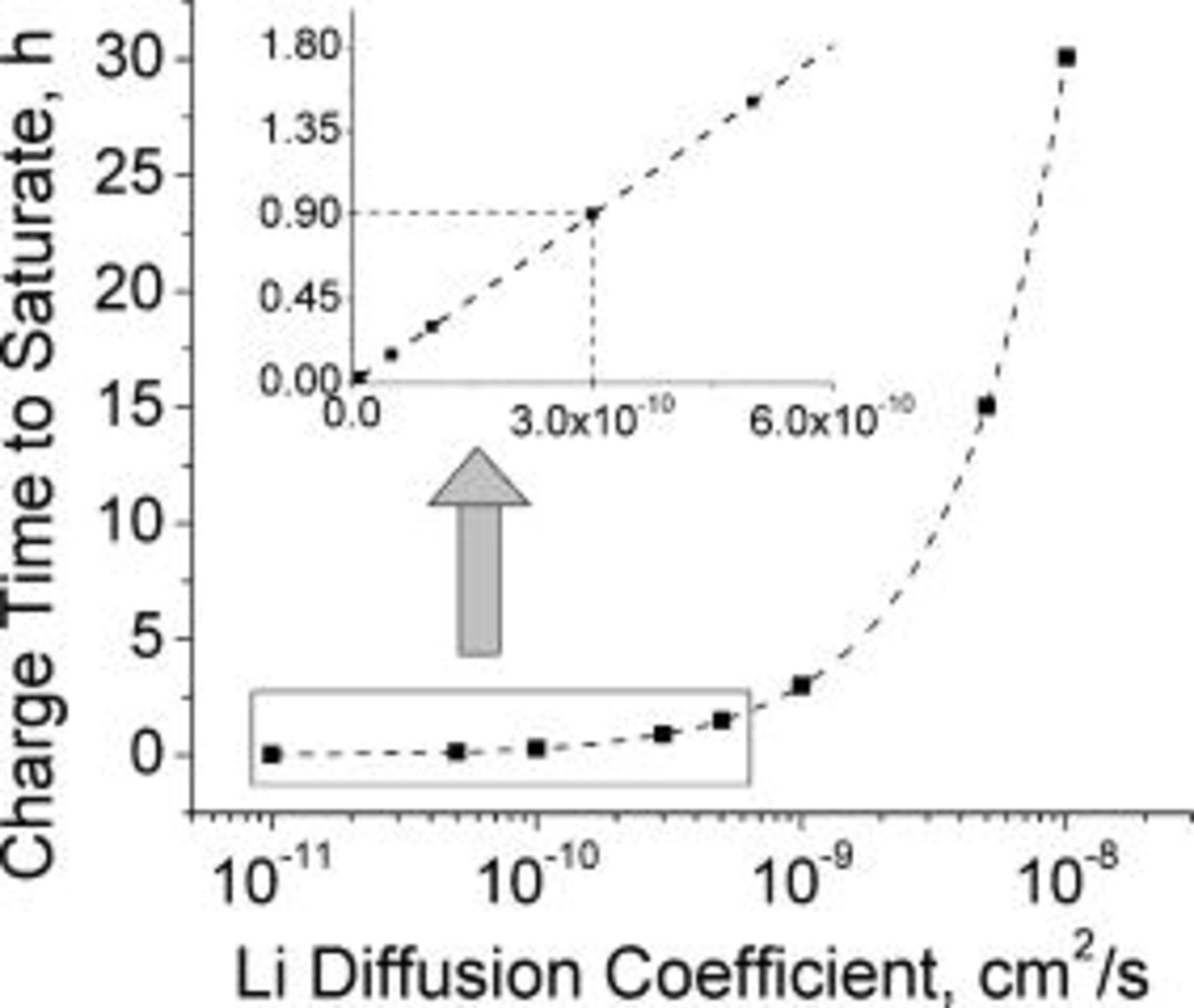
Figure 5. Maximal constant current charging time before metallic lithium is formed at the graphite∕SEI interface modeled as a function of the lithium diffusion coefficient. Lithium saturates in  for a diffusion coefficient of
  as shown in the inset. The graphite layer thickness is
  and the charging current density is
  (
( charging). The dotted line connects the simulated data points. The line in the inset appears linear because the inset
  scale is linear and covers only a limited range.
Figure 6. Charging time at constant current before metallic lithium is formed at the graphite∕SEI interface, modeled as a function of the charging rate. Rapid saturation of the lithium with increasing charging rates is indicated. The graphite layer thickness is  and the lithium diffusion coefficient is taken as
  . The dotted line connects the simulated data points.
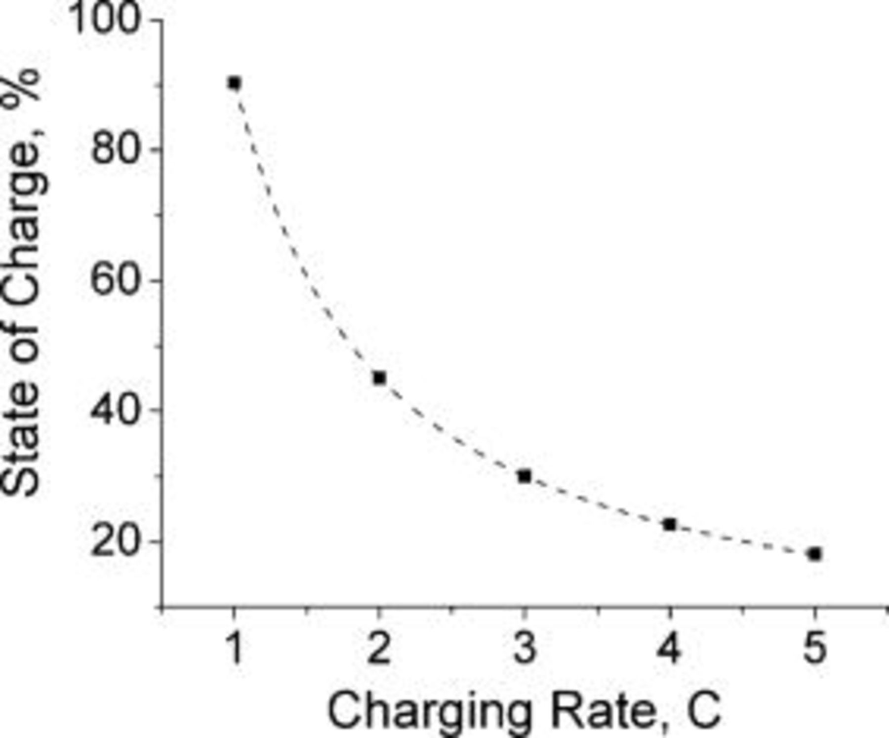
Figure 7. The modeled state of charge of the lithium-ion cell by the end of a constant current charging period (when lithium saturates) as a function of the charging rate. The state of charge decreases with increasing charging rate. The dotted line connects the simulated data points. The parameters are identical to those in Fig. 6.
Simulation and Discussion of Pulse Charging
Current pulsing, using special waveforms as shown below, can be used to increase the average diffusional flux of lithium into the graphite, thereby preventing metallic lithium formation and thus increasing the lithium-ion battery charging rate. A number of charging current waveforms are analyzed below.
Current pulsing with constant current amplitudes and constant pulse widths
Three different pulse sequences: (i) constant amplitude current pulses with constant rest periods (Fig. 8A); (ii) constant amplitude charge current pulses with periodic current reversal (Fig. 8B); and (iii) current pulses consisting of two different charge steps (Fig. 8C) were simulated. All these pulse sequences share as a common characteristic constant pulse widths and constant pulse amplitudes. As discussed earlier, the superposition principle23 was used to simulate the concentration profiles generated by the current pulses. The variation of lithium concentration at the graphite∕SEI interface as a function of charge time for a pulse sequence consisting of two different charge steps (Fig. 8C) is shown in Fig. 9. The two charge current densities,  and
and  , are 2.5 and
  , respectively. The two charge pulse widths,
  and
and  , are 3 and
  , respectively. The average current density of the pulse sequence encompassing the two different charge steps is
  and is identical to that of the conventional charging current density. The time to reach lithium saturation at the interface is
  (Fig. 9), same as the saturation time for constant current charging. The inset in Fig. 9 shows that the lithium concentration due to the applied pulse sequence oscillates about that of the constant current. Figure 10 shows that the total charge passed until the lithium reaches saturation is
  , identical to the charge passed by constant current of
  , corresponding to only 90% of the cell capacity. As noted in Fig. 9 and 10, no advantage in terms of postponing the lithium saturation at the interface is indicated. These results disprove the notion that pulse charging with constant current amplitudes and constant pulse widths offer advantage in terms of lithium battery charging rates.
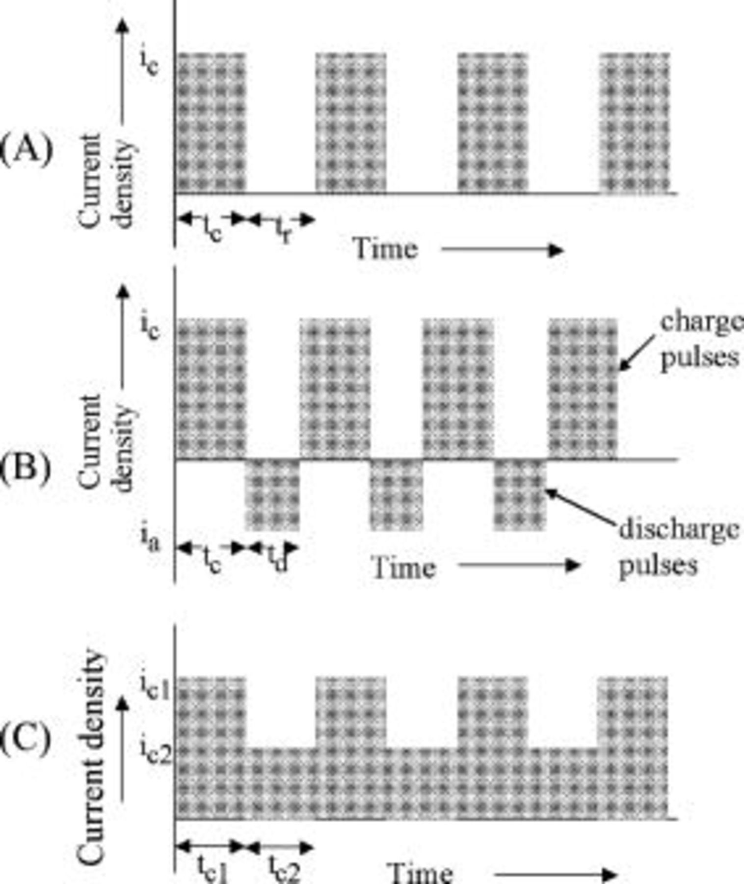
Figure 8. Schematic of different pulse sequences. (A) Constant amplitude pulsed current interspersed with identical rest periods; (B) constant amplitude pulsed current interspersed with alternating constant amplitude discharge pulses; and (C) pulsed current consisting of a sequence of different amplitudes charge current density pulses.
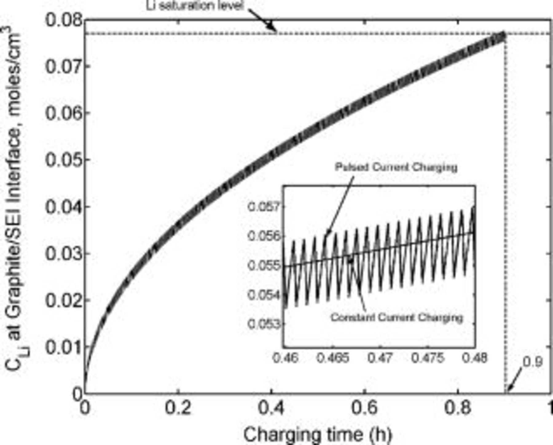
Figure 9. Lithium concentration at the graphite∕SEI interface modeled as a function of time during current pulsing. The pulse sequence consists of alternating two different amplitude charge current pulses (Fig. 8). The charge current densities,  and
and  , are 2.5 and
  , respectively, and the corresponding pulse widths are 3 and
  , respectively. Lithium saturates at the interface in
  , identical to the time for conventional constant current charging. The inset shows that the lithium concentration during current pulsing oscillates around that of the lithium concentration during constant current charging. The lithium diffusion coefficient is taken as
  .
.
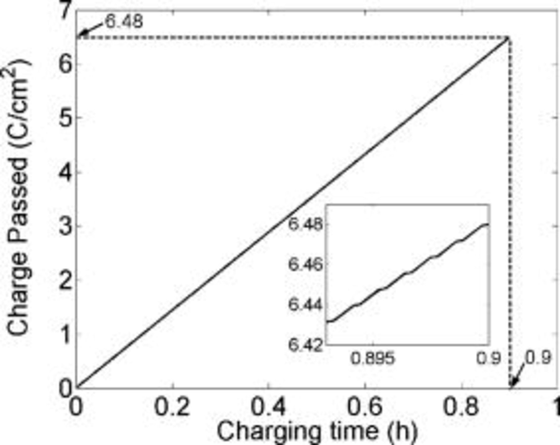
Figure 10. Charge passed per unit area modeled as a function of charging time during pulse charging following the sequence shown in Fig. 8C. The charge passed until saturation is reached is  , identical to that of the conventional current charging. Only 90% of the cell capacity is charged. All parameters and conditions are as indicated in Fig. 9.
The other current waveforms indicated in Fig. 8A and 8B were simulated at various duty cycles, current densities, and pulse widths, leading to the conclusion that current waveforms with constant current amplitudes and constant pulse widths offer no advantage. An in-depth study of theses waveforms was published earlier.23 In the following sections, pulse sequences with varying amplitudes or varying pulse widths are considered.
Current pulsing with constant current amplitudes and varying pulse widths
A pulse sequence of alternating charge and rest pulses as shown schematically in Fig. 11 is considered. A constant current density,  , is applied during the charging pulses with no current passing during the rest periods. The width of each charging pulse is selected as the time required for lithium to saturate, i.e., reach the concentration of saturated lithium,
  , at the graphite∕SEI interface. Each charge pulse is followed by a rest pulse. The width of the rest pulse is determined such that it provides sufficient time for the lithium concentration at the graphite∕SEI interface to relax to a preset concentration designated as the lower pulsing concentration,
  . This latter value is selected arbitrarily as some fraction of the saturated lithium concentration. Consequently, the lithium concentration at the graphite∕SEI interface oscillates during this mode of pulse charging between the saturation concentration (by the end of the charge or on pulse) and
  .
.
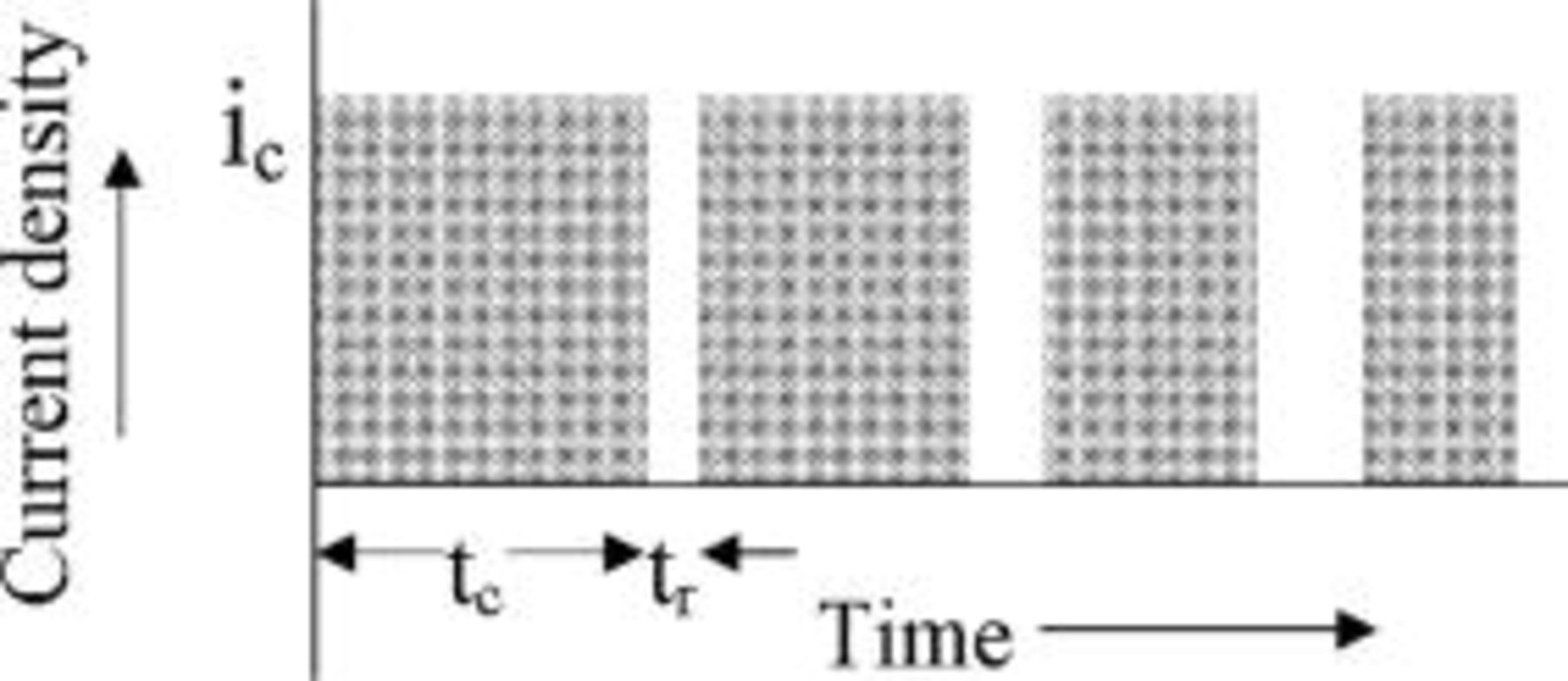
Figure 11. Schematic of constant amplitude pulsed current interspersed with rest periods. The charging pulse widths decrease and the rest pulse widths increase with time.
The superposition principle was used to simulate the concentration profiles generated by the current pulses. The diffusion equation 3 with appropriate initial and boundary conditions (Eq. 4, 5, 6) for the alternating current and the rest pulses was solved for a charging current density of  , lithium diffusion coefficient of
  , and a lower pulsing concentration,
  , of
, of  (78% of saturation). Figure 12 shows the modeled lithium concentration as a function of distance from the graphite∕SEI interface, at the end of the first charging pulse and the following rest pulse. The slope during the charge pulse at the graphite∕SEI interface
  in Fig. 12 is determined by the applied current density (Eq. 5). The slope is zero during the rest pulse as no current passes. Due to the relatively short rest time, only a small amount of relaxation is noted. As discussed later in more detail, such short relaxation times are advantageous as they minimize the charging period that is not used efficiently while still preventing the formation of metallic lithium at the interface.
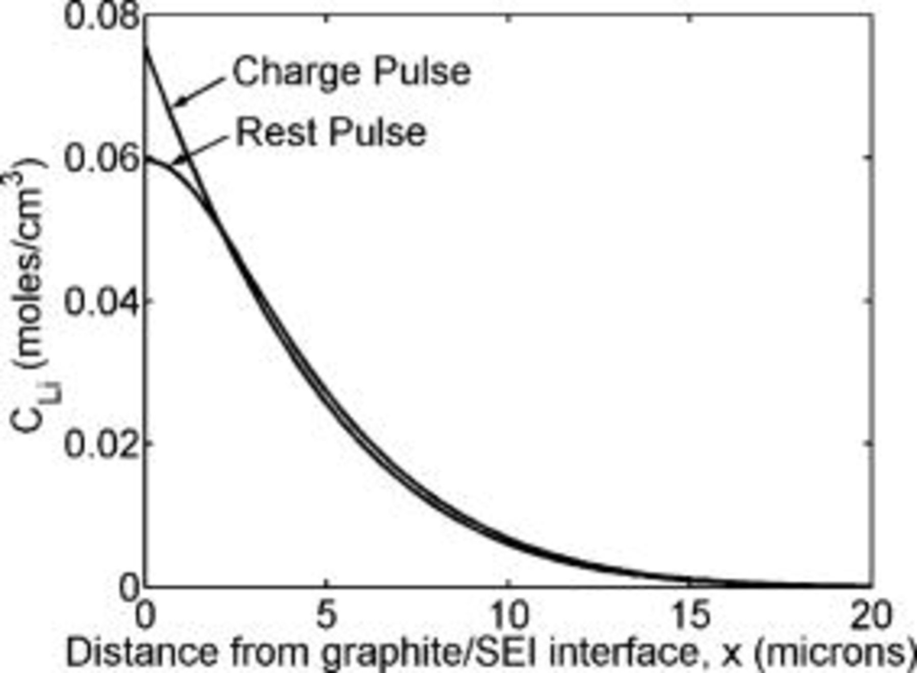
Figure 12. Lithium concentration computed as a function of distance from the graphite∕SEI interface at the end of the first charge pulse and the subsequent rest period. The charging current density is taken as  , the diffusion coefficient is
  , and the lower pulsing concentration,
  , is
, is  . Due to the short rest time, only a small amount of relaxation of the concentration profile is noted.
Figure 13 shows the modeled oscillations of the lithium concentration at the graphite∕SEI interface  between
  and
and  at the end of the charge and the rest pulses. It is evident that this type of pulsing (Fig. 11) prevents the formation of metallic lithium by allowing the lithium to relax during the rest pulse. Figure 13 also indicates that the width of the first charge pulse is longer than subsequent charge pulses because it takes a long time for the lithium concentration to build up to the saturation level. The shape of the concentration profile indicates that the rest periods increase (down-trending lines become less steep), while the charging pulse times decrease (upward trending lines become steeper) with the pulse number. This effect is due to the lithium concentration buildup inside the graphite layer, as discussed in more detail later.
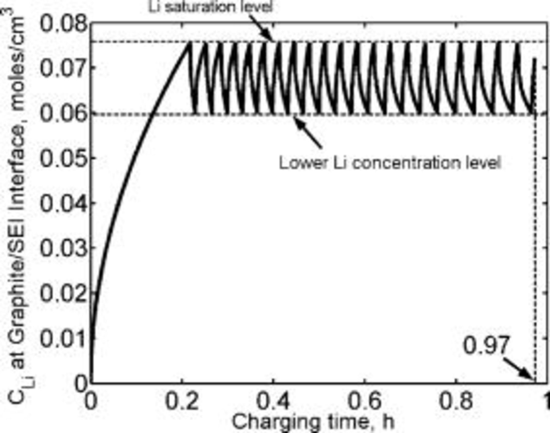
Figure 13. Lithium concentration at the graphite∕SEI interface modeled as a function of time during current pulsing oscillating between saturation and  . All parameters and conditions are as indicated in Fig. 12.
The nominal capacity of the lithium-intercalated graphite electrode in a typical Sony lithium-ion battery US18650S is  ,4 which is equivalent to
  . Figure 14 compares the simulated time required to charge the lithium-ion battery to
  by current pulsing following the protocol outlined above and by conventional charging. The lower pulsing concentration,
  , is taken as
  . The mode of current pulsing is as shown in Fig. 11 and the current density during the charging pulse is
  (
( rate). Conventional charging is modeled at a constant current density of
  (
( rate) until about
  , when the lithium concentration at the graphite∕SEI interface reaches the saturation level and is then followed by constant voltage charging. The current density during the constant voltage phase trickles down to low values (Fig. 1) and therefore charge passed during this time is low. It is evident from Fig. 14 that current pulse charging with varying charge and rest pulse widths, following the protocol listed above, is faster than conventional charging. It takes about
  to charge the lithium-ion battery by conventional charging, whereas it takes only about
  to charge the battery by current pulsing, following the protocol listed above.
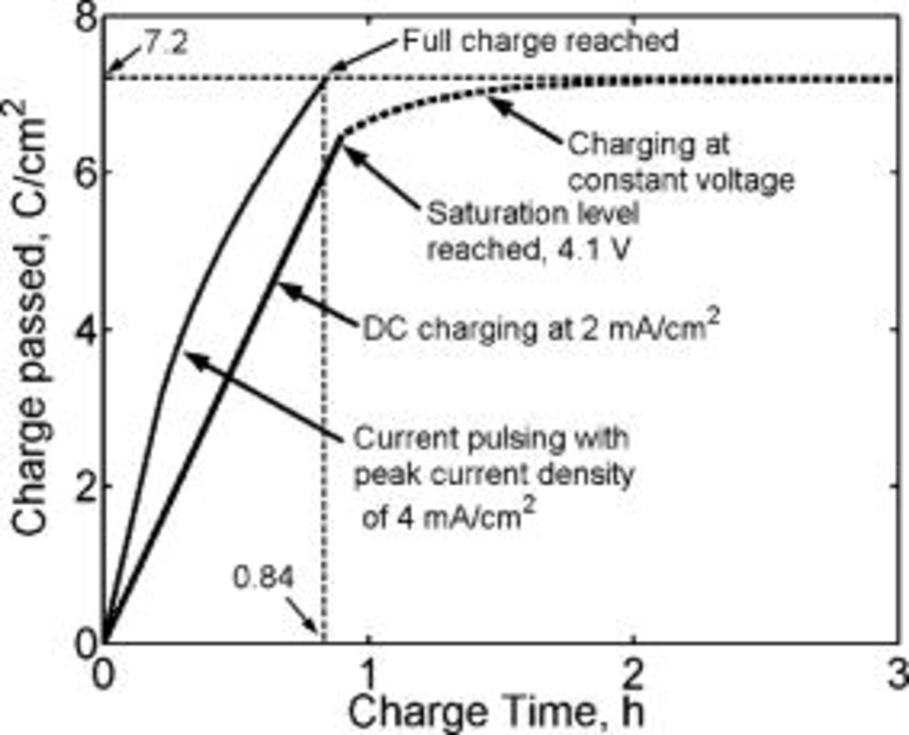
Figure 14. Comparison of simulated current pulse charging with varying charge and rest pulse widths following the sequence shown in Fig. 11, to conventional charging. The charging current density during the current pulses is  . The constant current density in conventional charging is
  . Saturation at the interface is reached in
  . The subsequent constant voltage charging phase (dotted line) is approximated. Current pulse charging is about 3 times faster than conventional charging (0.84 vs
  ). The diffusion coefficient is
  and the lower pulsing concentration is
  .
.
The lower pulsing concentration,  , is a preset arbitrary limit. The effect of changing this parameter on the charging time is shown in Fig. 15. The charging current density, the diffusion coefficient, and the graphite layer thickness were fixed at the values listed in Table I. Figure 15 shows the simulated amount of charge passed per unit area as a function of time for pulse charging following the protocol listed above, for three values of
  : 0.06, 0.065, and
  corresponding to 78%, 84%, and 91% of the saturation concentration, respectively. The modeling indicates that it would take only about
  to charge the lithium-ion battery completely when
  is set at
  (91% of saturation). In comparison, for lower pulsing concentrations of 0.065 and
  , it takes about 0.89 and
  , respectively, to achieve full charge. Comparing the data in Fig. 15, it is evident that the time required to fully charge the battery decreases with increase in the lower pulsing concentration. Clearly, maintaining the interfacial lithium concentration close to saturation (but not exceeding it) is beneficial because this provides the highest driving force for lithium diffusion away from the interface into the intercalant. The difference between
  and
and  may be viewed as a safety factor, which for fastest charging should be maintained as low as practically possible, without ever allowing the interfacial concentration to exceed
  . During the rest pulse, the lithium concentration at the graphite∕SEI interface decreases with time. The rate at which the concentration changes also decreases with the rest time. Therefore, applying a significantly much longer rest pulse width does not relax the lithium concentration at the graphite∕SEI interface much further. By increasing the lower pulsing concentration, the rest pulse width is decreased and therefore the time to fully charge the battery is shorter.
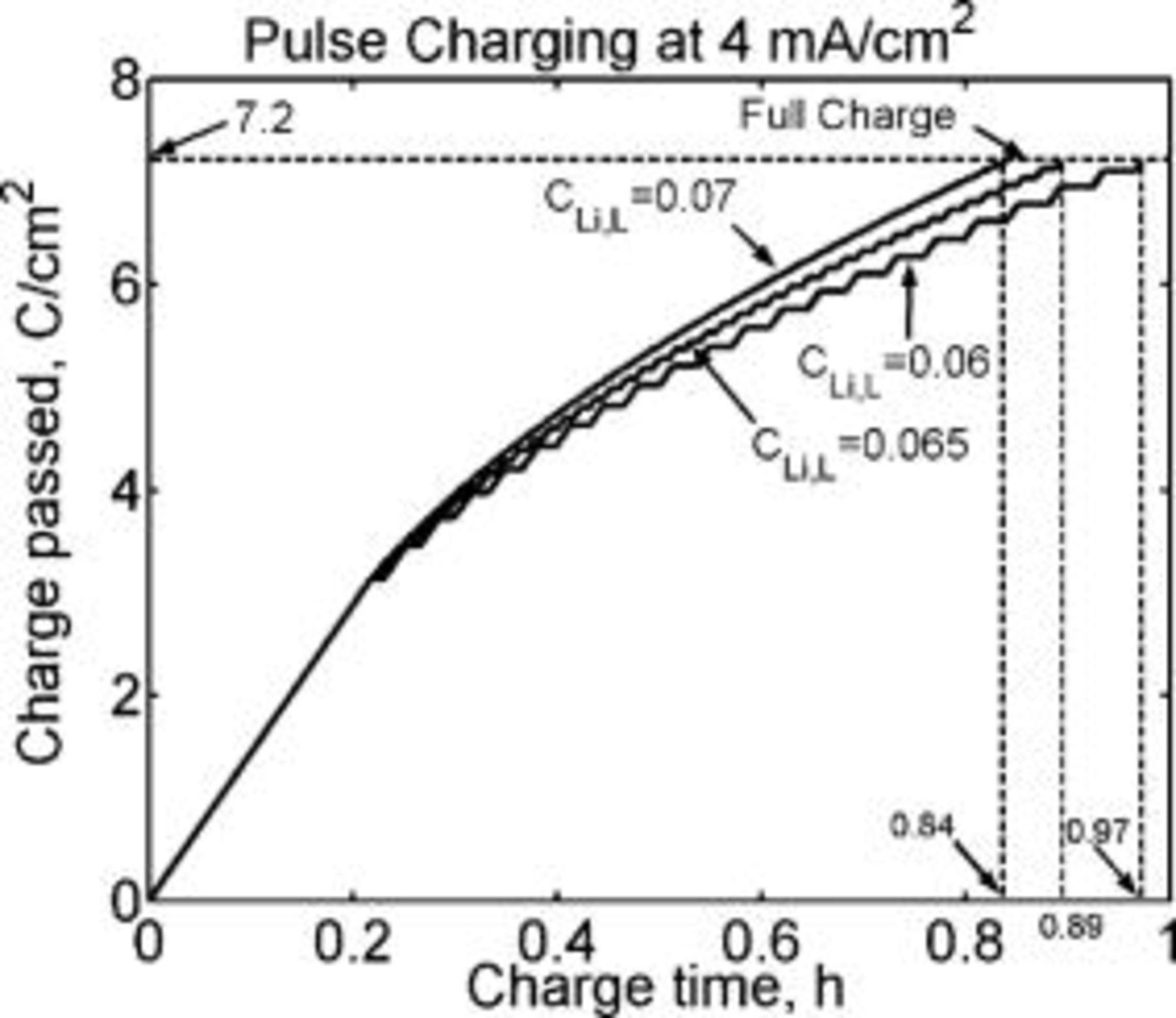
Figure 15. Charge passed per unit area modeled as a function of charging time during pulse charging following the scheme shown in Fig. 11 for three lower pulsing concentrations,  , of 0.06, 0.065, and
  . The charging current density is
  and the diffusion coefficient is
  .
.
Table I. Parameters selected for modeling the lithium diffusion into graphite.
| Parameter | Value |
|---|---|
Lithium diffusion coefficient, 
|
|
| Thickness of the graphite electrode, δ |
 (Ref. 20, 25) (Ref. 20, 25) |
| Charging current density |

|
The effect of the charging current density is studied by fixing all other parameters: the lithium diffusion coefficient to  ,28 the thickness of the graphite layer, δ, to
  ,20, 25 and the lower pulsing concentration to
  . The simulated charging times required to fully charge the battery for different charging current densities are listed in Table II. It is evident that the total charging time is about the same for all the charging current densities. This conclusion also holds true for the other lower pulsing concentrations studied (results not shown). This seemingly surprising result can be explained by the fact that the process rate is controlled by the lithium diffusion into the intercalant layer. When the applied current density is higher, the charging pulses must be kept shorter and the rest periods longer to avoid lithium saturation at the interface. At lower current densities the charging pulse can be longer and the rest periods shorter. Consequently, the average charging rate simulated for the different current densities is about the same.
Table II. Total charge time as a function of the peak pulse current density. The lower pulsing concentration is set at  .
.
Peak pulse current density 
| Total charge time (h) |
|---|---|
| 4 | 0.89 |
| 6 | 0.88 |
| 8 | 0.89 |
Current pulsing with varying current amplitudes
In the previous section, it was shown that current pulsing with varying pulse widths can charge the lithium-ion battery significantly faster than by conventional charging if the parameters are selected properly. The pulse widths were determined by maintaining the lithium concentration at the graphite∕SEI interface close to, but not exceeding, the saturation level. However, it is difficult to apply this protocol practically because monitoring the lithium concentration at the graphite electrode interface is not easy. Therefore, taking the cue from the previous analysis, we replicate the effects of the current pulsing with varying pulse widths by current pulsing with varying current densities.
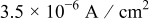
Consider the pulse sequence shown in Fig. 16. The pulse width of both the charging and the rest pulses is constant; however, the current density applied during each charging pulse is decreased as the pulse sequence progresses. The diffusion rate of lithium into the graphite at the graphite∕SEI interface is high at the start of the charging cycle when the intercalant is free of lithium, and then decreases with time as the lithium accumulates within the graphite. Therefore, a pulse-charging sequence was modeled where high current densities are applied during the initial charging pulses, when the diffusion rate is high. The current density is decreased as the sequence progresses to prevent lithium from saturating at the interface.
Figure 16. Schematic of pulsed current interspersed with rest periods. The magnitude of the charging current density decreases as the pulse sequence progresses. The charging and the rest pulses widths modeled here are constant.
We set as a goal to fully charge the lithium-ion battery in  without saturating the lithium at the graphite∕SEI interface. It was shown in the previous section that this is feasible. A duty cycle of 75% with charge pulse width,
  and rest pulse width,
  was considered. Selection of these values was based on recognizing that pulsing in the seconds range is sufficient to relax the lithium concentration in the battery. It was shown in the previous section that longer rest time is futile and only contributes to increasing the charging time of the battery. Based on the above values and the goal to fully charge the cell in
  , the average current density was determined. The parameters are listed in Table III. The decrease of the current density with the pulse number was selected to be linear according to

 is the total number of pulses and
  is the charging pulse number in the sequence;
  and
and  are constants listed in Table III. In this particular case, the charging current density was taken as

This corresponds to an initial current density of  , which drops linearly to
  at
at 
 .
.
Table III. Current pulsing parameters for charging the battery in  .
.
| Parameter | Value |
|---|---|
| Total charge time |

|
| Duty cycle | 75% |
Charge pulse width, 
|

|
Rest pulse width, 
|

|
| Total number of pulses | 1530 |
| Average current density |
|
Constant, 
|
|
Constant, 
|

|
The superposition principle23 was used to determine the concentration profile for current pulsing with time-varying current densities. Figure 17 shows the variation in the lithium concentration at the graphite∕SEI interface as a function of the charging time for the parameter set listed in Table III (corresponding to pulse charging in  ). It is evident from Fig. 17 that lithium never saturates at the interface during the entire charging cycle. Figure 18 indicates that a total charge of
  is passed in about
  . It is difficult to observe the small oscillations due to the current pulsing in the lithium concentration (Fig. 17) and the charge passed (Fig. 18) because the pulsing is of the order of seconds and the plotted time scale is of the order of hours.
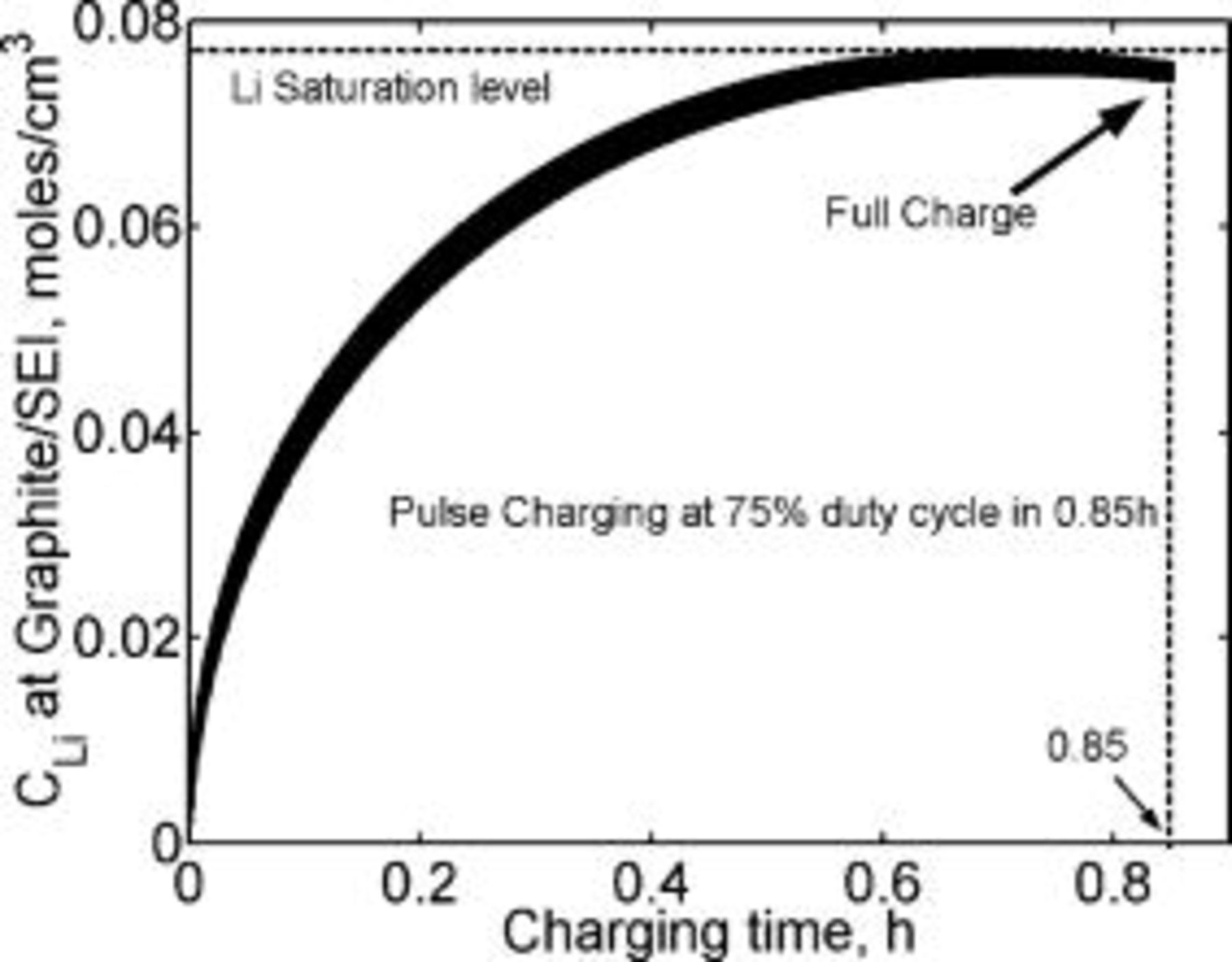
Figure 17. Lithium concentration at the graphite∕SEI interface modeled as a function of charging time for the parameter set listed in Table III. The total charging time is  . The line depicting the lithium concentration appears thick due to the high frequency pulsing.
Figure 18. Charge passed modeled as a function of the charging time for the parameter set listed in Table III. The total charging time is  .
.
It is evident from the above discussion and simulations that by selecting appropriate parameters for current pulsing, lithium saturation at the interface can be avoided while still providing high charging rates. Applying this method, the lithium-ion battery can be charged in about  , instead of the
  required by conventional charging techniques.
Simulation and Discussion of Nonlinearly Decreasing Charging Current
In this section, the variation of the mass transfer coefficient for lithium diffusion in graphite as a function of time is analyzed and the advantage of tracking the variations in the mass transfer coefficient by the current density to achieve high charging rate is illustrated.
Mass transfer coefficient for lithium diffusion
Considering for simplicity the semi-infinite diffusion of lithium into a graphite matrix instead of finite diffusion within a restricted region, and solving for a current step indicates that the lithium concentration at the graphite∕SEI interface,  increases according to29
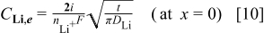
The lithium flux can be represented in terms of a mass transport coefficient 
Recognizing that  and
and  for diffusion into a semi-infinite region, we compare Eq. 10, 11 to obtain
Accordingly, the mass transfer coefficient decreases with the inverse of the square root of time, for a current step as shown in Fig. 19. It is evident that the mass transfer coefficient is high at small times because there is no lithium inside the graphite matrix at the start of charging. As time passes, the mass transfer coefficient decreases due to lithium buildup inside the graphite matrix.
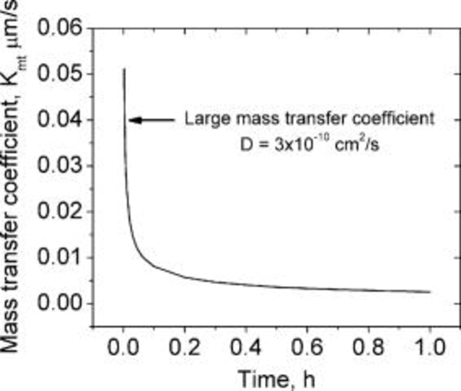
Figure 19. Mass transfer coefficient as a function of the charging time for lithium diffusion coefficient of  .
.  is large for initial times and decreases rapidly with time.
The current density is obtained in terms of the mass transfer coefficient by comparing Eq. 11, 12 with 
Equation 13 indicates a nonlinearly decreasing current density tracking the variation of the mass transfer coefficient in the graphite matrix. The current density is a function of the lithium diffusion coefficient and the lithium concentration at the graphite∕SEI interface,  . The lithium concentration at the interface is taken as the lithium saturation concentration,
 . Equation 13 was determined for semi-infinite diffusion and its application to finite diffusion was done with a slight adjustment of the saturated lithium concentration
  to assure that the interfacial lithium buildup according to the solution (Eq. 7) does not exceed
  . A more precise analysis for finite diffusion is possible; however, solving the diffusion equation 3 by applying the superposition principle for the precise conditions simulated is mathematically complex and unjustified here.
Nonlinearly decreasing current tracking the mass transfer coefficient
A nonlinear decreasing current profile following the trend indicated by the mass transfer coefficient was considered by applying Eq. 13 as shown in Fig. 20. The current density at the start of charging is large,  , and at the end of charging is
  , a value that is lower than the conventional charging current density
  . The lithium concentration at the graphite∕SEI interface and the charge passed during the application of the current waveform (Fig. 20) are shown in Fig. 21. The total charging time for this waveform is only about
  , lower than the charging times determined using the profiles described in the previous sections (current pulsing with constant current amplitudes and varying pulse widths and current pulsing with varying current amplitudes). The lithium concentration at the graphite∕SEI interface during this entire charging cycle is below the lithium saturation concentration. In fact, shorter charging times can be obtained by applying higher current densities at the start of charging. However, practical heat management issues may limit the charging current densities that can be applied to the lithium-ion cell.
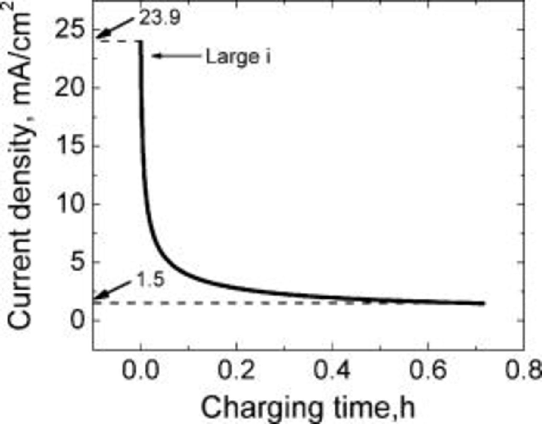
Figure 20. Nonlinearly decreasing current density profile modeled as a function of the charging time. The current density profile tracks the variation of the mass transfer coefficient for lithium diffusion. The initial charging current density,  , is much higher, while the final current density,
  , is lower than conventional charging current density.
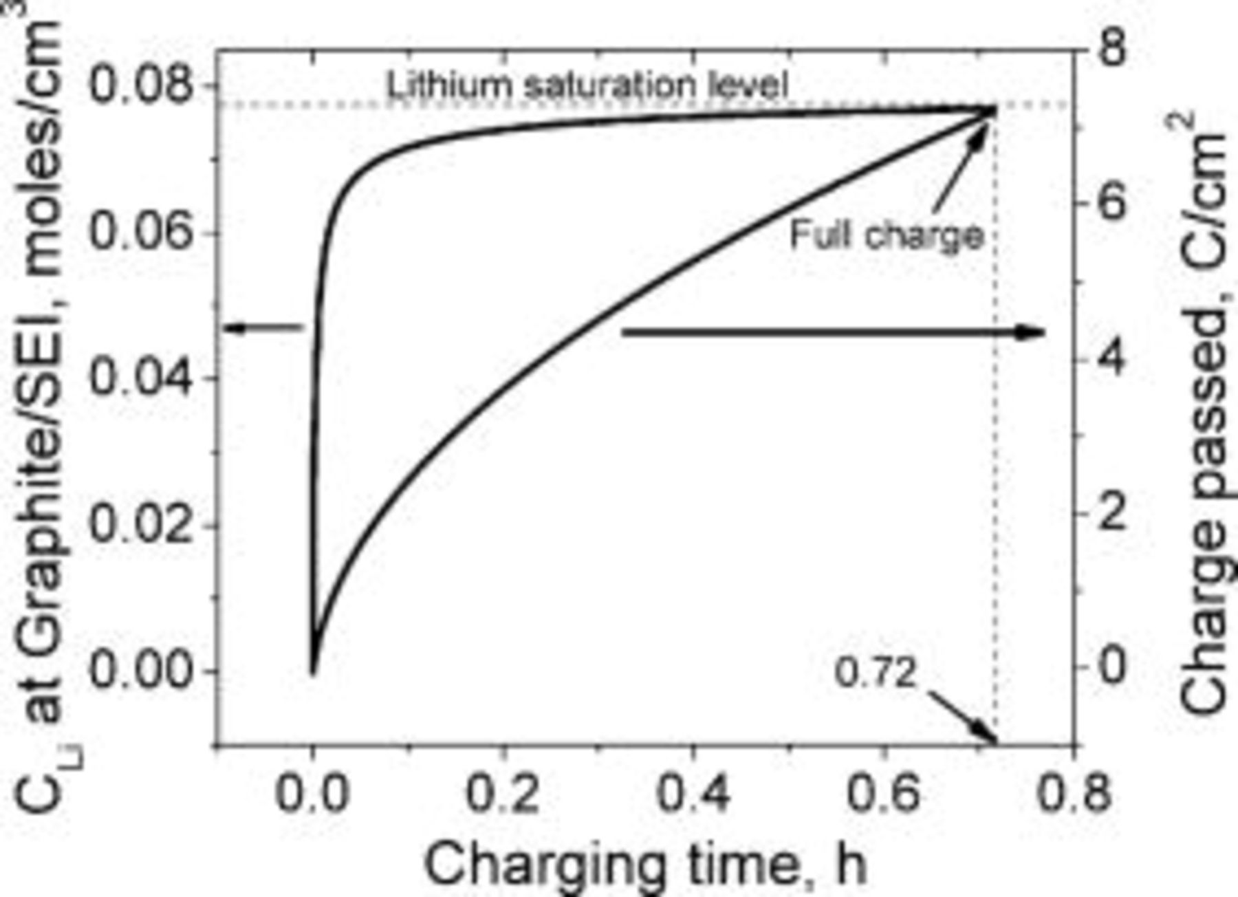
Figure 21. Lithium concentration at the graphite∕SEI interface and the charge passed modeled as a function of the charging time. The waveform of the modeled current density is shown in Fig. 20. The lithium concentration is always lower than the saturation level,  . The lithium-ion cell is shown to charge completely in just
  . The lithium diffusion coefficient is taken as
  .
.
It is evident from the above discussion that current pulsing with appropriate waveform may provide higher charging rates as compared to conventional charging while avoiding lithium saturation at the interface.
Conclusions
The lithium concentration builds up at the graphite∕SEI interface during the charging process of the lithium cell when applying conventional charging protocol. After a long (about  ) charging period at constant current, the lithium concentration at the interface reaches the saturation level, which requires switching from a constant current charging mode to a constant potential charging at a significantly lower average current density. This extends the charging time of the lithium-ion battery by about 2 additional hours.
To overcome this problem, a current pulse waveform with restrictions on the lithium concentration buildup at the interface was considered. The upper limit of the lithium concentration at the interface, which determines the charging pulse width, was set as  , just below the saturation limit. The lower limit of the lithium concentration at the interface (lower pulsing concentration), which determines the rest pulse width, was explored at different values of 0.06, 0.065, and
  . The proposed pulse sequence enables higher charging rates, without ever reaching lithium saturation, resulting in shorter charging times. The modeled pulse charging using the specific waveforms suggested was about 2.4–2.9 times faster than conventional charging.
A different pulse sequence with varying current densities (instead of varying pulse widths) was also modeled. The current density applied during the charging pulses decreased with the charging time. Simulations again show that the battery can be fully charged in about  .
.
Pulsing using the specific suggested waveforms is effective in enhancing the charging rate because it allows the lithium surface concentration to reach a high level early on in the charging cycle without, however, exceeding the saturation level. This provides the maximal diffusion rate. Later, as the concentration within the intercalant builds up, the charging current is decreased by lowering the magnitude of the current or by increasing the rest time during which the lithium concentration profile relaxes. This trend is required due to the decrease of the mass transfer coefficient with time. A nonlinearly decreasing current, tracking the variations in the mass transfer coefficient, was modeled resulting in a charging time of only about  , much faster than the other simulated pulse charging profiles. The only caveat is that the initial high charging rates may be limited by heat dissipation inside the lithium ion cell.
Following the methods illustrated above, simulations indicate that the lithium-ion battery can be fully charged in less than an hour, instead of the  required for conventional charging.
Acknowledgments
This research was supported by ENREV Inc. Helpful discussions with Professor Morrison, Jr., Dr. Tibor Kalnoki-Kis, and Dr. Han Wu are acknowledged.
List of Symbols

| constant listed in Table III, 
|

| constant listed in Table III, 
|

| lithium concentration, 
|

| bulk lithium concentration, 
|

| lower pulsing lithium concentration, 
|

| saturated lithium concentration, 
|

| lithium concentration at the graphite∕SEI interface, 
|

| lithium diffusion coefficient, 
|

| Faraday constant, 
|

| current density,  or or 
|

| number of eigenterms |

| mass transfer constant, cm∕s |

| number of electrons transferred in lithium-ion reduction, equivalents∕mole |

| lithium formation flux, 
|

| lithium diffusion flux, 
|

| total number of pulses |

| number of charge pulses |

| time, s |

| distance from the graphite∕SEI interface towards the graphite interior, cm |
Greek
| δ | thickness of graphite intercalant layer, cm |