This chapter applies the tools of the previous chapters to a particular company, Inditex, the largest fast fashion company in the world. The fast fashion industry faces major social (S) and environmental (E) challenges. Moreover, since the industry is characterised by high levels of outsourcing, those challenges tend to be hidden down the supply chain. The case study answers questions such as: how to calculate the integrated value of a company? Which company-reported data to use? How to fill the gaps from missing data in company reporting? We connect the company’s business model and purpose to its external impacts and transition challenges. This allows us to value on environmental (E), social (S), and financial (F) factors. We compute the company’s integrated value (IV) by summing FV, SV, and EV in several ways. The company’s IV turns out to be positive overall, but both positive SV and negative SV and EV turn out to be much larger than FV, which shows the importance of not netting. The large negative values need to be addressed: to be reduced and ideally eliminated. We therefore explore integrated value creation over time; how it can be improved; and how to communicate it to investors.
Overview
This chapter applies the tools of the previous chapters, such as the equity valuation models of Chap. 9 and the social and environmental valuation models of Chap. 5, to a particular company. It is a case study that gives an external perspective on the integrated value of Inditex as of January 2021 for educational purposes. It answers questions such as: how to calculate the integrated value of a company? Which company-reported data to use? How to fill the gaps from missing data in company reporting?
Inditex, or Industria de Diseño Textil, S.A., is a multinational clothing company, based in Arteixo, Spain. It is the largest fast fashion company in the world and operates over 7000 stores in almost 100 countries. The company is best known for its Zara brand, but also owns brands such as Bershka, Massimo Dutti, Pull&Bear, Zara Home, and Oysho. The fast fashion industry faces major social (S) and environmental (E) challenges. Moreover, since the industry is characterised by high levels of outsourcing, those challenges tend to be hidden down the supply chain.
Anzeige
In the following sections, we briefly introduce the nature of the company’s activities and its value drivers. We then connect the company’s business model and purpose to its external impacts and transition challenges. This allows us to value the company in various ways.
First, we make an assessment of its financial value F, including the effect of sustainability issues (inward view, Sect. 11.3), in several scenarios. We use the discounted cash flow (DCF) model for calculating F.
Second, we estimate Inditex’ value on S and E (outward view, Sect. 11.4), with flows projections on S and E, similar to those of an ordinary DCF. These calculations indicate that there is significant value destruction on E and S, but also significant value creation on S.
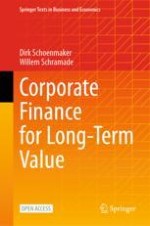
Third, we compute the company’s integrated value (IV) by summing FV, SV, and EV in several ways (Sect. 11.5). The company’s integrated value turns out to be positive overall, but both positive SV and negative SV and EV turn out to be much larger than FV, which shows the importance of not netting. The large negative values need to be addressed: to be reduced and ideally eliminated. We therefore explore integrated value creation over time; how it can be improved; and how to communicate it to investors. See Fig. 11.1 for a chapter overview.
A chart represents 4 sub-topics of Chapter 11 sustainability unaware, including basics and valuation of private equity, E S G integrated or inward view including the impact of S and E in private equity, and impact or outward view and integrated value in private equity.
Fig. 11.1
Chapter overview
×
Anzeige
Learning Objectives
After you have studied this chapter, you should be able to:
link a company’s business model to its external impacts and transition exposures
build a company valuation model that incorporates F, S, and E
create and interpret a company value creation profile
assess corporate investments on F, S, and E in the context of the company’s value creation profile
critically assess a company’s information provisions on sustainability issues and the gaps therein
11.1 Introduction to Inditex
Inditex, officially known as Industria de Diseño Textil (which translates to ‘Textile Design Industry’), is a Spanish clothing company with a large portfolio of global fast fashion brands such as Zara, Bershka, Pull&Bear, and many more. With more than 7200 stores in 93 countries it is the biggest fast fashion group in the world.
In 1975, Amancio Ortega and his wife Rosalia Mera opened their first fashion store for their brand Zara. Later that year, Ortega hired a local professor, José Maria Castellano, who would be responsible for growing the company’s computing capabilities. In 1984, Castellano was appointed CEO after having developed a revolutionary design and distribution method that greatly improved the company’s performance. A year later Inditex was created as a holding company for Zara and its production facilities. After expanding internationally by opening a store in Portugal in 1988, the company started developing other brands such as Pull&Bear in 1991, Lefties in 1993, and Bershka in 1998.
When Inditex had its IPO in 2001 at the Spanish Stock Exchange, the company was valued at €9 billion. Over the course of the 2000s the company experienced exponential growth, achieving a milestone 2000 stores in 2004 and 4000 stores in 2008. In the meantime, Castellano was replaced by current CEO Pablo Isla in 2005. While the company has grown to become the largest fashion retailer in the world, it was hit hard by the Covid-19 pandemic as the company saw its revenue decrease by 27.7% in 2020.
The company operates a number of brands but the Zara and Zara Home brands still account for more than two-thirds of sales. Geographically, the company’s sales are skewed to Europe (over 60%, of which 25% in Spain), with significant presences in Asia-Pacific (25% of sales) and the Americas (14% of sales).
Inditex claims to employ a ‘multi-concept strategy’, with ‘market segmentation through distinctive concepts’; independent management teams; a global presence; and the same business model across all concepts—i.e., with a high frequency of new collections; and outsourced production in low-cost countries. The business model is discussed further in Sect. 11.2.
Like any industry, the fast fashion industry is exposed to trends that affect its growth and the way it operates. According to the international consultancy PwC, the industry’s key trends are sustainability and digitalisation.1 For example, 3D design was quick to substitute fashion shows when those were no longer possible due to Covid-19 restrictions. Meanwhile customers are becoming more critical about clothing companies’ sustainability performance, and they demand better information on the footprint of individual pieces of clothing. As a result, supply chain transparency is becoming more important and increasingly enabled by digitalisation.
Company Value Drivers
The financial valuation analysis (Sect. 11.3) starts with Inditex’s value drivers: sales, margins, and capital. Table 11.1 shows Inditex’s sales. Inditex has produced consistent growth numbers during the 2010s with a minor blip in 2013, due to additional investments in refurbishing flagship brands and opening many new stores globally. The lower growth at the end of the decade indicated to some, including Morgan Stanley, that the company’s growth profile was fading.2 While this could have played a part in the devastating sales drop in 2020, it should be largely attributed to the effects of the Covid-19 pandemic which saw a staggering drop in sales globally due to lockdown measures. However, with global fashion sales in 2020 declining between 15 and 30%, Inditex seemingly took a larger hit than most.3
Table 11.1
Sales of Inditex (in billions of €)
A table has values for sales in euro billions and sales growth for the years 2011, 2012, 2013, 2014, 2015, 2016, 2017, 2018, 2019, and 2020.
Inditex’s profitability has been remarkably consistent throughout the last decade, especially in terms of EBIT which ranged from 16.7 to 19.6% over the course of 9 years (see Table 11.2). The company’s EBITDA has also performed well, although decreasing slightly over time. The strong increase in EBITDA in 2019 compared to 2018 is furthermore noticeable. This indicates that, although the company strongly improved its gross profit, there was also a significant growth in depreciation considering that EBIT stayed the same. The increased depreciation can be attributed to the 30.9% growth in assets during 2019.
Table 11.2
Profitability of Inditex (in millions of €)
A table has values for E B I T euro millions, E B I T margin, E B I T D A in euro millions, and E B I T D A margin for the years 2011, 2012, 2013, 2014, 2015, 2016, 2017, 2018, 2019, and 2020.
Except for 2020, Inditex showed a strong financial performance over the past decade. Inditex’s growth during the last decade is noticeable in the development of its assets, which has more than doubled since 2010 (see Table 11.3). In fact, assets grew faster than sales (falling sales-to-assets ratio), possibly indicating that the company is operating less efficiently than before. For most of the decade, its sales-to-assets ratio was around 1.2, which is similar to other companies in the fashion sector, such as H&M. In contrast to other financial numbers, Inditex’s capex (investments) has been relatively inconsistent, particularly from 2017 onwards. In 2020 the capex was even negative, which means the company divested some of its assets. Finally, the Return on Assets has been healthy.
Table 11.3
Capital of Inditex (in millions of €)
A table has values for total assets, sales slash assets, capex, capex slash sales, and R O A for the years 2011, 2012, 2013, 2014, 2015, 2016, 2017, 2018, 2019, and 2020.
11.2 Inditex’ Business Model and Transition Challenges
Ultimately, to value Inditex on F, S, and E, we need to understand the company’s external impacts and transition challenges. This in turn requires an understanding of the company’s business model and purpose.
11.2.1 Business Model
In both its company profile and its 2020 Annual Report (AR 2020), Inditex spends several pages explaining its business model. Inditex claims to have a unique business model, ‘fully integrated, digital and sustainable’. But is it? And how can it be described in a more objective way? As discussed in Chap. 2, Johnson et al. (2008) argue that a successful business model has three components:
1.
A customer value proposition: the model helps customers perform a specific ‘job’ that alternative offerings do not address;
2.
A profit formula: the model generates value for the company through factors such as the revenue model, cost structure, margins, and/or inventory turnover;
3.
Key resources and processes: the company has the people, technology, products, facilities, equipment, and brand required to deliver the value proposition to targeted customers. The company also has processes (training, manufacturing, services) to leverage those resources.
For Inditex, these three components can be described as shown in Fig. 11.2.
A chart represents three components of the business model. These are customer value proposition, profit formula, and key resources and processes. Each component enlists related elements.
Fig. 11.2
The three components of Inditex’ business model. Note: Authors’ assessment based on Annual Report 2020. At Inditex (and many other companies) sales/invested capital (IC) is higher than sales/assets, since invested capital is lower than total assets, from which short-term liabilities are deducted (and networking capital added) to arrive at IC
×
Crucially, Inditex’s customer value proposition is driven by frequently issuing new collections. To minimise costs and maintain high levels of ROIC, the garments are produced in an outsourced supply chain over which the company exercises strong bargaining power but limited control. This means large negative external impacts can be created beyond the boundaries of Inditex’ legal entities4—and indeed they are, as we will see later on. Strengths from an F perspective can be weaknesses from an S and E perspective. Box 11.1 provides a critical perspective on Inditex’s marketing.
Box 11.1 Sustainable Marketing
Fuller (1999) defines sustainable marketing as ‘the process of planning, implementing, and controlling the development, pricing, promotion, and distribution of products in a manner that satisfies the following three criteria: (1) customer needs are met, (2) organisational goals are attained, and (3) the process is compatible with ecosystems’.
The above definition is over 20 years old, and with current knowledge one could argue that the third criterion should be refined to ‘within social and planetary boundaries’. However, that does not change our judgement: that Inditex succeeds at criteria (1) and (2) while failing at (3).5 To stay within planetary boundaries, Inditex has to adjust its marketing mix, do serious product system life cycle management, and broaden its view on customer value. This could mean switching to a model with lower product volumes, longer product lives, and selling fashion as a service, renting or leasing clothing instead of selling it. Such new models would cannibalise the company’s existing models, which makes it a tough call for management. Still, it probably makes sense to at least do this in an experimental way alongside the current model, and the company seems to have started on this journey.
11.2.2 Purpose
A company’s purpose is the reason for its existence, which is grounded in the way it creates value for its clients and other stakeholders. Hence, it should be closely related to its business model and competitive position. In the case of Inditex, it is hard to find a stated purpose.
The word purpose is mentioned 79 times in the 2020 Inditex Annual Report but only once in the meaning that we are looking for—and that instance is in a table on page 581 of the report, in reference to its annual corporate governance report. In the latter report, the word purpose is used 83 times, but again only once in the meaning we are looking for, in a section on board responsibilities (page 167): ‘Monitoring compliance with the company’s internal codes of conduct and corporate governance rules, also ensuring that the corporate culture is aligned with its purpose and values’. However, the purpose itself is not mentioned.
The closest we find is this excerpt from the company’s ‘About us’ section: ‘Our workforce never loses sight of the customer. We work to create value beyond profit, putting people and the environment at the centre of our decision-making, and always striving to do and be better. It is fundamental to how we do business that our fashion is Right to Wear’.6 And for the Zara brand, the website says: ‘Bringing attractive and responsible fashion, as well as improving the customer’s experience, are Zara’s priorities’.7
Hence, Inditex’ purpose is a question mark. And so is the fit of that purpose with what stakeholders want, and with what is needed for successfully navigating transitions.
11.2.3 Stakeholders
Value is created for a multitude of stakeholders. But who are the company’s main stakeholders? And how do their interests relate to and conflict with each other? Like many companies, Inditex gives an overview of its stakeholders (as identified by Inditex itself) in Fig. 11.3.
A graphical representation of Inditex's stakeholders. Customers, employees, suppliers, the community, the environment, and shareholders are among them.
Fig. 11.3
Inditex’s stakeholders according to Inditex. Source: Adapted from Inditex Annual Report 2020, page 42
×
The company also gives an overview of the associated tools for dialogue. However, the friction between stakeholders is not given—and one might even disagree with the list of identified stakeholders. It is therefore useful to fill out a stakeholder impact map, as done in Table 11.4.
Table 11.4
Stakeholder impact map for Inditex
A table with three columns and 7 rows. The column heads are stakeholders, goals, and helped or hurt. A few entries from the third to fifth row in the third column are highlighted.
Note: Authors’ assessments. We identify roughly the same stakeholders as Inditex does, but some with different labels as the scope is slightly different
The boldly framed box in the stakeholder map shows the main frictions: those with nature, the company’s suppliers, and the employees of its suppliers. These are the result of the company’s business model. First, the outsourced supply chain means that costs are minimised at the expense of suppliers, who in turn minimise their costs at the expense of environmental costs and their employees. Second, the high frequency of new collections, transported over large distances, and whose leftovers are burned impose a very high environmental cost.
So far, the relation with customers seems to be fairly comfortable, but that is changing too: Neumann et al. (2020) find that perceptions of social responsibility directly affect consumers’ attitudes towards fast fashion brands, as well as trust (a direct predictor of purchase intention) and perceived consumer effectiveness. Apparently, consumers need to perceive sustainability efforts of these brands as altruistic.
11.2.4 Financially Material Sustainability Issues
The stakeholder impact map gives good clues about the company’s financially material sustainability issues: the issues that could or indeed already do affect the company’s financial value drivers. Figure 11.4 gives an overview of the issues that Inditex deems material.
A two-part table has three columns and seven rows. The column headings are number, material topic, and subtopics.
Fig. 11.4
Inditex’s material issues according to Inditex. Source: Adapted from Inditex Annual Report 2020, page 70
×
Some of these issues are purely on the E side (e.g., climate change; environmental footprint minimisation; protection of natural resources), some purely on the S side (e.g., diversity, equality and inclusion; quality of employment; human rights), while others are overarching or a mix of both (e.g., value chain transparency and traceability; value creation; ethical behaviour and governance).
It is hard to disagree with the above material issues, but that doesn’t mean that they take them seriously enough. Inditex could cherish minor improvements on these issues while shunning the elephant in the room. For example, the practice of cancelling already produced goods is at odds with both ethical behaviour and responsible purchasing. And there seems to be very little progress on topics such as circularity and value chain transparency & traceability.
What is missing from the analysis is a clear view on how these topics relate to each other. Unfortunately, the company doesn’t apply the concept of double materiality (i.e. clearly distinguishing how material issues affect Inditex—the inward perspective of Fig. 11.4) and how Inditex creates external impacts8 (the outward perspective). And hence the feedback loop between internal and external impacts is not discussed (see Chap. 2 on double materiality).
11.2.5 External Impacts (Outward Perspective)
External impacts are typically not a company’s favourite topic (as it often has a negative public relations effect), but it is very important to society: what kind of positive and/or negative external impacts does the company generate? To what extent does the company report about these external impacts? Can they be quantified, or even be priced? Remember that for both SV and EV, the value calculation can be done in the three steps as presented in Chap. 5:
1.
Materiality assessment: determine important S and E factors
2.
Quantification: express these factors in their own units (Q)
3.
Monetisation: express these factors in money with shadow prices (SP)
In this section we take step 1 for Inditex; steps 2 and 3 follow in Sect. 11.4.
Be mindful that we present ways for outsiders (i.e. those without access to the detailed information that people within the company have) to value EV and SV. The company itself can go much further and in much more detail. It can actually compile impact-weighted accounts, i.e. an impact-weighted P&L and an impact-weighted balance sheet. The Impact Economy Foundation (2022) gives guidance on how to do that in its Impact-Weight Accounts Framework (IWAF) and provides principles accordingly (see Chap. 5). It takes the perspective of a company or an auditor, that means it emphasises precision, whereas we take the perspective of an investor or stakeholder who wants to have rough understanding. Some organisations, such as Alliander and ABN AMRO in the Netherlands, have already published impact statements in the spirit of the IWAF statements (see Chap. 17).
As an investor or stakeholder, our first objective is the same as in the IWAF framework: identification of material impacts. As shown in Appendix A5.1 of Chap. 5, IEF (2022) provides a list of impact categories, which we map to the Inditex business model in Table 11.5. We also add planetary boundaries impacts that are not included in IWAF. This assessment is based on multiple sources, such as sustainability research articles by asset managers, sustainability ratings agencies, and NGOs; and academic literature on sustainability in textiles and fashion.
Table 11.5
Likely external impacts created by Inditex’ business model, by IWAF impact category
Key impact categories
Likely positive or negative
Problematic if substantially negative
Profit
P
Salaries
P
Interest payments
P
Taxes
P
Payments to suppliers
P
Payments from clients
N
Cost of capital
N
Change in fixed assets
?
Client value of products
P
Client value of services
N/A
Value of impact materials
N
Potentially
Creation of intellectual capital
P
Well-being of employment
?
Potentially
Value to employees due to training and experience
P
Effects on human health
N
Potentially
Occupational health & safety incidents
N
Potentially
Time invested by employees
N
Contribution to/limitation of climate change
N
Potentially
Contribution to/limitation of pollutiona
N
Potentially
Contribution to/limitation of availability of scarce natural resourcesb
N
Potentially
Contribution to/limitation of poverty
Both
Potentially
Contribution to/limitation of human rights violations
N
Potentially
Source: Authors’ analysis based on the Impact-Weight Accounts Framework (IWAF; IEF, 2022)
aIncluding nitrogen & phosphorus cycles
bIncluding deforestation, freshwater use, and biodiversity loss
Most of these issues are recognised as problems by Inditex. And the company has some goals on these topics, such as 100% eco-efficient stores and removal of plastics bags. However, the issues are discussed without putting them in the proper context and without being clear about the size of these problems. As a result, it is impossible to tell how close or far off these targets are in reducing the company’s harm to (almost) zero. In fact, it turns out they do not even come close, as we will see later on, since these goals and all current efforts are mainly on the company’s own operations, and not the vastly larger operations in its supply chains.
Fortunately, some context is given. In its Annual Report, Inditex describes some initiatives, for example, on circularity: ‘Under the Make Fashion Circular initiative, Inditex has participated in developing a common circular economy framework for fashion, which has been integrated into our strategy’ (AR, 2020, p.280). And it says this on GHG emissions (AR, 2020, p.319): ‘Inditex has set ambitious emissions reduction targets approved by the Science Based Target Initiative (SBTi), which envisage a 90% reduction in Scope 1 and 2 emissions and a 20% reduction in Scope 3 (purchased goods) emissions, in both cases for the 2018-2030 period. These targets are the first milestone in Inditex’s ambitious emissions reduction strategy, whose purpose is to achieve decarbonisation by 2050’.
The trouble though is that Scope 3 is what matters most, since Scope 3 accounts for about 98% of the company’s total emissions.9 Hence, the company’s focus on the least significant part is misleading and taints the credibility of its sustainability ambitions.
11.2.6 Transition
Inditex’ negative external impacts are the main sources of the company’s transition risks and opportunities. The x-curve of transition in Fig. 11.5 illustrates them by showing the current regime (top left) of fast fashion at the lowest possible prices; the emerging niches (bottom left), such as responsible fashion, second hand, recycled, and rented clothing, which provide the ingredients for the desired future regime (top right) of responsible & circular fashion; the bottom right gives examples for practices that need to be phased out, such as the burning of unsold clothing.
A schematic of an x curve. The top left represents fast fashion at the lowest prices and the top right presents responsible and circular fashion at fair and real prices. The bottom left exhibits responsible fashion and the bottom right mentions the burning of unsold clothing and cancellation of orders.
Fig. 11.5
X-curve of transition for Inditex and fast fashion. Note: Filled in for the fashion industry by the authors; adapted from Loorbach et al. (2017)
×
The question is how Inditex is going to navigate this transition. How quick and broad-based is the transition of the fast fashion sector? Can it significantly reduce its negative impacts without perishing in the process? How well prepared is Inditex compared to others? To what extent can Inditex adapt? The answers to these questions can be expressed in an estimate for parameters bj and ai from Eq. 2.1 in Chap. 2.
Given the major negative impacts that the fast fashion industry generates for society on both S and E and the availability of substitutes, we rate the industry’s transition exposure (bj) quite high at 0.8. This means that a large part of the industry is likely to be transformed. On the adaptability of both the industry and the company (ai), we take a more mixed view. On the one hand, there is plenty of scope to mitigate social issues in the supply chain; the company could stop burning clothes; and there are opportunities in adopting alternative business models based on better customer information, rental and recycling. On the other hand, the high frequency of new collections is such an integral part of the business model that one could question the company’s (and the industry’s) ability to really reduce its negative environmental impacts. And so far, this seems to remain out of scope. Thorisdottir and Johannsdottir (2020) find that CSR managers within the industry focus on supply chain innovation, eco-friendly products, and workers’ safety. There are some sustainable fashion brands, but they are mostly small or medium-sized (Triodos Investment Management, 2021).
11.2.7 Management
The above considerations raise the question of management quality. Management has been very successful in growing the company in a profitable way. Operational excellence and customer centricity are major strengths. But the transition challenges demand a rethinking and redesigning of the business model. ‘What got you here, won’t get you there’. The key question is whether management is up to that challenge. The company’s reporting suggests that management is still partly in denial, but strategic thinking tends to be ahead of reporting. Next, the company does experiment with alternative business models in, for example, recycling. Will it dare to allocate more resources to such strategic options? Will it dare to cut value destructive activities that are currently cash flow positive? These are the questions that investors and other stakeholders should be asking.
Interestingly, there is a change in management, with Óscar García Maceiras being named the new CEO, and Marta Ortega Pérez, the founder’s daughter becoming the new chairwoman. A BBC news item is sceptical on her appointment:10 ‘She says she’s grown up around the company and learned a lot in her time formally working there. But others will see this more as a Spanish version of the hit HBO series “Succession”, where family members are given preference for top jobs over better qualified members of the team. Indeed shares in Inditex have fallen on news of the appointment’. The item also refers to a number of challenges that management faces: ‘At a time when consumers are becoming more aware of the environmental costs of fast fashion, Zara particularly is in an awkward spot—its reputation is built on bringing style trends to High Street stores quickly and cheaply. There are also supply chain concerns. In November 2021, authorities in the French city of Bordeaux rejected plans by a Zara store to double its floor space, over allegations the fashion label may have profited from the forced labour of Uighurs in China. But the new chief executive and chairwoman are unlikely to be steering the Inditex ship without the help of founder Amancio. When he resigned as chairman in 2011, he didn’t put his feet up. Instead the man known as “The Boss” has remained very much involved in the company. Though now aged in his 80s, it’s a fair bet he’ll remain so, even with the appointment of the new executive team’.
11.3 Valuing Inditex in Financial Terms (Inward Perspective)
What does this all mean for the valuation of Inditex’ financial value? Let’s take a step back and look at a basic valuation model for the company. To be clear: this section is only about F. As far as E and S are included, it is about their impact on F. This is the inward (or ESG integration) perspective. The next section takes the outward perspective and values E and S.
11.3.1 Basic Model: Before Assuming a Transition
As argued in Chaps. 6 and 9, the best method for valuing F is a DCF analysis. One can build a DCF from scratch in Excel or use a template in which the model is already prebuilt, including the formulas that relate the cells to each other. Table 11.6 shows such a template, filled out for Inditex per 1 January 2021. In the model, the grey cells represent historical data or assumed historical data that are filled in for the specific company; the black cells are assumptions; and the white cells give results from formulas. For example, the 2017 taxes on EBIT are the product of the 2017 EBIT (historical data) and the 2017 effective tax rate (assumed historical). The value driver assumptions are expressed in growth rates (such as sales growth) and ratios (such as the EBIT margin), where the historical ones (here 2017–2020) provide an indication for the value driver assumptions. For example, the 2017–2019 EBIT margins (and further back) give a good impression of what normal EBIT margins for Inditex look like, hence our 16.5% EBIT margin going forward..
Table 11.6
Basic DCF for Inditex
A basic D C F dataset. It mentions values of value driver assumptions in the categories of historical, assumptions, and calculated. It also represents values for W A C C and T V growth.
Filling in the historical data is relatively straightforward, but making the assumptions requires making choices. One way to do that is to extrapolate the past into the future, i.e. take growth and margin assumptions that are simply the average of historical growth and margins. However, that’s a naïve approach, especially for companies that have been growing very fast in the past and/or had very high margins.
Our preferred approach is to reverse-engineer the DCF to the current stock price. I.e., what growth, margins, and cost of capital does the share price imply? This is effectively the market’s opinion, which one can contrast with one’s own assumptions. So, the 0% upside is not a coincidence, but by design: we made adjustments to the value driver assumptions in such a way that they resulted in a fair share price that equals the (then) current share price. This can deliver interesting information: sometimes the market prices in value drivers are much more aggressive than the historical ones, which could be a sign of overvaluation or of very good business prospects; other times, the forward-looking value drivers are much more modest than the historical ones, which could be a sign of undervaluation or of declining business. In the case of Inditex, the market seems to agree that its growth will slow down but that it can maintain its high margins.
Next to sales growth and margins, the cost of capital is the third value driver (see Chap. 9). We use the weighted average cost of capital (WACC) provided by Eq. 13.4 (see Chap. 13):
whereby rE is the cost of equity and rD the cost of debt. Chap. 12 explains in more detail how to calculate the cost of equity and debt. The basic idea is that the cost of equity is a combination of a risk-free rate rf and a premium for market risk (E[rMKT] − rf). The exact cost of equity depends on a company’s sensitivity to market risk, which is called the βi. So, we only need to calculate the beta from market data (see Chap. 12 how the beta can be derived from the correlation of a company’s stock returns with the stock market). We find a beta βi of 1.21, based on 5-year monthly stock returns. The risk-free rate rf of 1.5% and the market risk premium (E[rMKT] − rf) of 5% are generally applicable parameters. Using Eq. 12.15, we get rE = rf + βi ∙ (E[rMKT] − rf) = 1.5 % + 1.21 ∗ 5 % = 7.6%.
For the cost of debt, we can add the credit risk premium to the risk-free rate. Inditex has an AA credit rating, which is equivalent to a credit risk premium of 1% (see Chap. 12). So, the cost of debt is rD = rf + AA spread = 1.5 % + 1.0 % = 2.5%.
Table 11.6 shows that equity E is €82.2 billion and net debt D is −€3.1 billion (as Inditex’s cash position is higher than its debt load). Using Eq. 9.1, we can calculate the enterprise value of the company V = E + D = €82.2 − €3.1 = €79.1 billion. Using Eq. 11.1, Inditex’s cost of capital is \( WACC=\frac{E}{V}\bullet {r}_E+\frac{D}{V}\bullet {r}_D=1.04\ast 7.6\%-0.04\ast 2.5\%=7.8\% \)
The company’s net debt is negative. With such low and negative leverage, the company’s share price has relatively low sensitivity to the value driver assumptions, which tends to make the model more reliable. Nevertheless, one should do several checks to the model to avoid mistakes. For example, one could check sensitivities of the DCF value to value driver changes; do a multiples analysis; and check for behavioural biases such as extrapolation and overoptimism.
11.3.2 Value Driver Adjustments
One way to link sustainability to valuation is by means of value driver adjustments (VDAs, see Chap. 9). In that method, the financially material issues are assessed in terms of their impact on value drivers in three steps:
1.
identify and focus on the most material issues;
2.
analyse the performance and impact of these material factors on the individual company; does the company perform better or worse on them than competitors do?
3.
quantify competitive advantages to adjust for value driver assumptions;
For example, in the case of Inditex one could argue that the company grows faster (i.e. higher share value) because of customer relations and innovation and that the cost of capital should be higher (i.e. lower share value) because of environmental issues. These views can be summarised in a table (like in Box 9.3 in Chap. 9) that gives the adjustments per value driver (sales growth, margins, and capital) per material issue, and how much they affect the fair value of the DCF. In this way, the analyst can argue why they value the company more or less due to sustainability issues. This is a powerful way to link sustainability to valuation. It is also very useful for comparing competing companies. The limitation of the VDA approach, however, is that it is still quite static, in that it does not explicitly take transitions into account. This is particularly important for companies, like Inditex, whose business models have so far been a strength, but are turning into a liability, which they already are in social and environmental terms.
11.3.3 Transition Valuation Scenarios
Qualitative transition scenarios can be deep and multifaceted, allowing management to identify new pathways for navigating transitions. Valuation scenarios, however, need to be simple to allow for quantification that makes intuitive sense. Table 11.7 describes such simple scenarios, along two dimensions: whether or not effective global climate mitigation occurs by 2030; and whether the company is well prepared for it.
Table 11.7
Transition valuation scenarios for Inditex
Effective global climate mitigation by 2030 (successful transition)
Mere climate adaptation, no serious mitigation by 2030 (unsuccessful transition)
Company is well prepared for climate mitigation
Scenario 1a: serious investment in recycling and in rental models; cutback on new collections; more ownership in the value chain
Scenario 2a: strategy as in 1a, but with less payoff
Company is ill-prepared
Scenario 1b: continued to operate in business-as-usual mode, missed trends, and paid high price
Scenario 2b: strategy as in 1b, but at no penalty
To get to a scenario weighted valuation, we need to make models for each scenario and assign probabilities to them. We assign a 40% probability to effective global climate mitigation by 2030, and a 60% probability that Inditex is well prepared for it. Note however that this is not necessarily a good thing, since in scenario 2a the company prepares for a transition that does not happen. Hence, the probability of scenario 1a is then 40%*60% = 24%. The probabilities of the other scenarios can be calculated through the same method. Table 11.8 shows how the valuation model differs per scenario, and what (probability-weighted) fair value results from all four scenarios together.
Table 11.8
Transition scenarios weighted valuation for Inditex
Scenario
DCF fair value per share
Probability
Main value driver assumptions (baseline from the basic scenario: 4.5% growth; 16.5% EBIT margin; 4% capex/sales)
1a (well prepared; successful transition)
€28.4
24% (60%*40%)
3 years of 3% growth rate, then back to 4.5%
3 years of 13% margins, then 20%
3 years of 6% capex/sales, then back to 4%
1b (ill-prepared; successful transition)
€10.4
16% (40%*40%)
−20% growth in 2023 and −15% growth in 2024, then 0% onwards*
3 years of 8% margins, then 11%
2a (well prepared; unsuccessful transition)
€22.5
36% (60%*60%)
10 years of 3% growth rate
3 years of 13% margins, then back to 16.5%
3 years of 6% capex/sales, then back to 4%
2b (ill-prepared; unsuccessful transition)
€31.9
24% (60%*40%)
6% sales growth
18% margins
Overall
€24.2
Note: Authors’ assumptions. *Of course, we could also model the drop to come later, much closer to 2030, with the same valuation impact. And yes, much worse scenarios are possible, in which the company fully misses the trend and fails
The most unfavourable scenario is 1b, in which the Inditex fair value is only €10.4 per share, versus €31.9 in the most advantageous scenario (2b). The weighted average fair value of all four scenarios is €24.2, which is below the January 2021 Inditex share price, suggesting that the company is overvalued. The overvaluation may be caused by not (sufficiently) considering the effect of E and S issues on financial value by most market analysts (see the adaptive markets hypothesis in Chap. 14).
Of course, all this is debatable, and people might differ in their opinions about the scenarios and their probabilities. In that sense, valuations are just opinions, and the market price is the aggregate of those opinions. Those who think that scenario 1b has a higher probability than the above 16% will likely arrive at a lower overall value for Inditex than our €24.2. And this is just the value of the Inditex share, i.e. an expression of the value of F. It does not say anything yet about the company’s value in terms of E and S.
11.4 Valuing S and E at Inditex (Outward Perspective)
For valuing S and E, we would ideally have the same level of detailed information that we have on F. At present, however, we are still far removed from that level. For most companies, GHG emissions are available to some extent, but company level data on the other planetary boundaries are typically missing. On S, indicators are often given, but typically only in relation to a company’s own operations; and reference to the SDGs is usually made, but not data that is actually useful in establishing the company’s contributions to (not) achieving them. As we will see, Inditex is no exception in that it does provide quite some data, but not of the right nature to value S and E.
To arrive at calculating SV and EV, we proceed on the path taken in Sect. 11.2, where we took the first of the below three steps:
1.
Materiality assessment: determine important S and E factors;
2.
Quantification: express these factors in their own units (Q);
3.
Monetisation: express these factors in money (SP)
11.4.1 Quantification: E and S in Their Own Units
When expressing E and S in its own units, we ideally obtain an overview like the one in Table 11.9, that is having yearly amounts for various types of E and S, both historically and projections for the coming years. The list is based on the issues identified in the External impacts part in Sect. 11.2.
Table 11.9
Expression of E and S in their own units
A table of expressions of E and S in their own units. The columns for the years, 2018, 2019, 2020, and 2030 have question marks in the rows.
Actually filling out a table like Table 11.9 is quite difficult: in practice, most companies only give historical data for some types of E; and then only for their own operations, not for their value chain. And for forward-looking data, they might give guidance or targets on, for example, GHG emissions. Indeed, for Inditex we find some historical numbers for 2019 and 2020 in the annual report, as well as some targets. For the 2021–2030 projections, we aim to make estimates based on relations with other company KPIs and company targets. The projections need to be linked to the company’s activity levels. This link is imprecise: we can use sales as a proxy, and then ideally only the volume component of sales, so excluding price; but even then, there might be a mismatch between production volumes (which tend to drive emissions and other impacts) and sales volumes. In fact, Inditex discloses the amount of garments it places on the market, which is a proxy for sales volume.
In Table 11.10, we try to quantify the impacts that Inditex makes and start out with the activity levels, which help to put E and S into perspective. Unfortunately, this is a very sobering exercise: we only find usable data for GHG emissions. And even there the picture is clouded by the company’s focus on Scope 1 and 2 (which is in direct control of Inditex), as it effectively hides its much larger Scope 3 emissions in its supply chain (98 to 99% of its total emissions) at the back of its AR 2020.11 Its ‘main decarbonisation commitments’ involve reducing Scope 1 and 2 by 90% by 2030, but the more important Scope 3 only by 20% by 2050—the company focuses on the former, while the latter is what matters.
Table 11.10
E and S in their own units
A table of E and S in their own units has a list of production and energy use in the years from 2017 to 2031. Certain rows of uses have only question marks.
Our assumptions are set accordingly, with a 2.5% annual reduction in Scope 3 emissions. This still results in 9.5 million tonnes of Scope 3 emissions by 2050. The other issues remain a series of question marks, for which we can look for proxies in external sources, which we will do in the next sub-section on monetisation.
The question marks mean that these impacts are not reported in the company’s disclosure, which raises the question to which extent the company considers them. After all, the company’s clothing products require cotton plantations, which use large amounts of water and nitrogen. There are emissions in transport and storage. And there is the waste generated across its supply chain, of which the company does report Scope 1 and 2, but not Scope 3; and does not split by waste type, which makes the data useless for our purposes. This also makes it impossible to determine the attribution of E and S: to what extent are they attributable to this company, and to what extent to other parts of the value chain?
Hence, the question of the user of an annual report should not just be: what’s in the company’s annual report? It should very much also be: what should be in their annual report that is currently not there? And how to communicate to the company that it should include it? As a rule, this amounts to timeseries data on the company’s contributions to planetary and social boundaries, ideally in a way that is relatable to its operations volumes. The guiding principle is double materiality: inwardly and outwardly material social and environmental factors should be included.
11.4.2 Monetisation: E and S in Monetary Terms
The third step to arrive at calculating EV and SV is monetisation, which is the expression of impacts in monetary units. To do so is challenging, especially if the non-monetary units are missing. But even then it can be done. The Impact-Weighted Accounts Framework (IWAF) (IEF, 2022) provides monetisation factors or shadow prices, which can be multiplied by the original units to arrive at monetary values. Table 11.11 lists some of IWAF’s shadow prices—see Appendix A5.1 for a full list of shadow prices with explanations.
Table 11.11
Examples of shadow prices, 2021
Key impact categories
Monetisation factor
Well-being of employment
$2647 per life satisfaction point (scale 0–100)
Effects on human health
$119,000 per DALY (disability-adjusted life year)
Occupational health & safety incidents
Fatal occupational accidents: $3,540,000 per accident
Occupational injuries with breach of H&S standards: $3840 per accident
Contribution to/limitation of climate change
$224 per tonne of CO2 equivalent (eq)
Contribution to/limitation of pollution—air pollution
Human toxicity: $119,000 per DALY
Nitrogen deposition NH3 from animal husbandry: $18.10/kg NH3 eq
From Table 11.11, we can directly apply the shadow price for contribution to climate change, which is €204 (=$224/1.1) per tonne of CO2 equivalent in 2021. The carbon price is projected to increase with 3.5% per year (see Chap. 5). Total emissions (the top line in Table 11.12) are taken from Table 11.10. Following IEF (2022), we assume that Scope 3 carbon emissions are 50% attributable to Inditex, as primary company in the supply chain (see Chap. 5). Table 11.12 shows how the resulting flows are calculated and discounted at the social discount rate of 2.2% (see Chaps. 4 and 12) to arrive at the present value of Inditex’s contribution to climate change, which amounts to −€101.3 billion.
Table 11.12
E flows and EV for climate change
A table of E flow and E V for climate change has a list of values of E flow energy change in the years 2020 to 2031. It includes factors that contribute to climate change, the cost of emissions in Euro billions, and the sum of P V in Euro billions.
Of course, that large negative number is a result of the assumptions we made (still resulting in 9.5 million tonnes of CO2 equivalent, as stated in Sect. 11.4.1), which are in turn driven by Inditex’s targets. For the other environmental and social issues, we lack the required data and cannot make such specific calculations. The rest of E is not there or hard to attribute (e.g., waste), and so is all of S. Hence, we don’t have the volumes of units to multiply with the monetisation factors. This applies not just to Inditex but is also typical for most companies. So, for the remaining issues we need to take shortcuts, such as using data of comparable companies or industry averages. In this case, we look for apparel data elsewhere. A publication by Impact Institute (2019) on the true price of jeans is quite helpful. Table 11.13 lists the components of the true price of jeans.
Table 11.13
Components of the true price of jeans
A table of components of the true price of jeans has 2 sections, namely S and E. It lists cotton cultivation, denim textile production, jeans manufacturing, transport, and total. The values of S total, E total, and total S and E are at the bottom.
The data from Table 11.13 allow us to calculate the proportions of negative S and E impacts in the true price of jeans, which we can extrapolate to apparel in general and Inditex in particular. We admit that this is a stretch, but it is the best we can do now given our current information.
Table 11.14 provides the proportions of E and S in the true price. The top panel expresses the amounts as percentage of E, which is €10.9 (see E total in Table 11.13). The first line shows the GHG emissions (climate change) from Table 11.13 as a percentage of E: 15% (=€1.61/€10.9). The second line shows the S total for each stage of the production process in Table 11.13 as a percentage of E: 202%. So, total S is twice as high as total E.
Table 11.14
Proportions of E and S in the true price of jeans
A table of proportions of E and S in the true price of jeans. It lists the values for cotton cultivation, denim textile production, jeans manufacturing, transport, and total.
The bottom panel expresses E and S as a percentage of the sales price, which is €80 per jeans. The GHG emissions are 2% (=€1.61/€80) of sales. Other E are 12% of sales. To prevent overestimation, we include only 50% of bonded labour in the S calculation, which is 20% of sales.
The above can be projected on Inditex in several ways. For example, we could assume that the other E impacts (i.e. E excluding GHG emissions) are 12% of sales of €29.6 bn in 2021 (Table 11.6): €3.5 bn per year. Or that the other E impacts are 6× larger than GHG emission impacts of €2.0 bn in 2021 (Table 11.12): €12.0 bn per year. However, we also observe that GHG emission impacts as a percentage of sales are much higher at Inditex (7% of sales, calculated as € 2.03 bn from Table 11.12 divided by €29.6 bn from Table 11.6) than in jeans (only 2% of sales in Table 11.14). This is partly due to much higher carbon prices, but does not fully explain the difference. We therefore feel that it’s better to stay on the lower side and go with the 12% of sales assumption for the other E impacts.
Next, we give Inditex the benefit of the doubt that it will materially bring down that number over time, with a 4% annual improvement. In addition, we assume that they are only 50% attributable to Inditex (as we do in Table 11.12). After all, not all these emissions are directly due to Inditex’ activities; a part is at suppliers—although then too, Inditex shares part of the responsibility. Chapter 5 explains that 50% of the E and S effects should be attributed to the integrated valuation of Inditex, as primary company in the supply chain, and the other 50% to the integrated valuation of other companies in the supply chain. Based on these assumptions, we calculate total E flows in Table 11.15. They amount to circa −€3.7 bn per year and a total EV of −€182.5 bn.
Table 11.15
Calculating E flows and EV for Inditex
A table of calculation of E flows and E V for Inditex. The values of E flows from 2020 to 2031 are listed. Total E flows in euro billions and the sum of P V in euro billions are highlighted.
For calculating S flows, we take a similar approach. The results are shown in Table 11.16. In the true price of jeans, S accounts for 28% of sales. However, that number is inflated by a very high number for bonded labour, which accounts for over half (€11.95 out of €22.20) of the negative S in the true price of jeans. To be on the conservative side, we take only half of that amount for the negative impacts of apparel. We arrive at negative S impacts of 20.3% of sales attributable to Inditex, which we apply in Table 11.16. Again, we give Inditex the benefit of the doubt that it will materially bring down that number over time, with a 4% annual improvement. We also attribute 50% of the negative S impacts to Inditex, because part of the negative S impacts occur at suppliers for which Inditex bears some responsibility as primary company in the supply chain. Based on these assumptions, we calculate total S flows in Table 11.16. They amount to circa −€2.9 bn per year and total negative SV of −€137.2 bn.
Table 11.16
Calculating negative S flows and negative SV for Inditex
A table of calculation of negative S flow and negative S V for Inditex. The values of negative S flows from 2020 to 2031 are listed. Total negative S flow in euro billions and the sum of P V in euro billions are highlighted.
The above numbers only include the negative S impacts of Inditex. However, the company also creates positive S impacts, such as the client value of its products (on top of what people pay for them), taxes, and the well-being of employment. The calculation of positive SV is shown in Table 11.17.
Table 11.17
Calculating positive S flows and positive SV for Inditex
A table of calculation of positive S flow and positive S V for Inditex. The values of positive S flows from 2020 to 2031 are listed. Total positive S flow in euro billions and the sum of P V in euro billions are highlighted.
Paid taxes of €0.5 billion were 2.2% of sales in 2020,12 but that number is not representative due to the Covid-19 pandemic. The corporate tax expense amounted to about €1.0 billion in the preceding years, or 3.7% of sales. The property and environmental taxes were 0.6% of sales. Combining the taxes, we arrive at a tax rate of 4.3% of sales.
The consumer surplus is a measure of consumer welfare and is defined as the social valuation of a product in excess of the price actually paid. As explained in Chap. 5, the consumer surplus is calculated as \( \left(\frac{Sales}{Price\ elasticity\ of\ demand}x\frac{1}{2}\right) \). Khaled and Lattimore (2006) find an average price elasticity of men’s and women’s clothing of 3.452. In the case of Inditex, the consumer surplus amounts to €2.955 billion (=€20.4 billion/3.452*0.5). This value has been created together by Inditex and its supply chain partners. We assume that the consumer surplus is 50% attributable to Inditex (and can be included in its integrated valuation), i.e. €1.478 billion, or 7.2% of sales.
The well-being of employment refers to additional well-being experienced by employees resulting from their employment at the company. We assume two life satisfaction points of €4813 (=2*$2647/1.1) (see Table 11.11). If we apply this to Inditex’ workforce of 144,116, we arrive at €694 million, or 3.4% of sales. However, since 2020 was a year with dramatically lower sales (i.e. inflating employees/sales), we have to correct this number for the lower sales of 31% in 2020 (which is a combination of a 28% drop in sales combined with an average sales growth of 3%) and use 2.3% (=3.4%*[100%–31%]) from 2021 onwards.
Adding up these numbers gives positive S flows of 13.9% of sales, which is over €4 billion per year—and growing; and a positive SV of €282.9 billion. Admittedly, positive SV benefits from growth, whereas negative SV (and negative EV) are based on more or less stable flows, since the reductions are already partly factored in.
Again, the above numbers are based on very rough assumptions, and hence very imprecise. However, they are the best estimate we have at this stage. And they point the way forward towards better data. For example, having academic evidence on the social value of apparel could help us make better assumptions. This applies even more strongly to data disclosed by the company on E and S in their own units.
11.5 Integrated Valuation of Inditex
Now that we have calculated estimates of EV and SV, we can calculate the company’s integrated value with Eq. 1.4 from Chap. 1: IV = FV + b ∙ SV + c ∙ EV. Figure 11.6 provides a schematic overview of the IV calculation.
A chart represents F value drivers, S in its own units, and E in its own units leading to F V, S V, and E V, respectively. These combine to form I V.
Fig. 11.6
Towards IV
×
As indicated in Chap. 6, the integrated value calculation can be done in several ways. We can add up FV, SV, and EV with equal or differing weights; and we could vary those weights depending on the sign of the values. In the basic IV model with equal weights (b = c = 1), we get IV = FV + SV + EV. For Inditex we then arrive at an integrated value (IV) of €42 billion for 2021, as shown in Table 11.18 and Fig. 11.7. Inditex’s integrated value is about half of its financial value of €79 billion.
Note: FV is the company’s enterprise value, which is the sum of equity and debt value
A positive-negative bar graph plots Inditex integrated value estimate. The positive S V has the highest Inditex integrated value estimate and the negative E V has the lowest.
Fig. 11.7
Composition of Inditex’s IV in basic IV model (b = c = 1)
×
Given the nature of the data and assumptions, these numbers are very rough estimates. But they do give a clear indication of the health (or lack thereof) of Inditex’s business model. The IPV is still positive, which means that on a net basis, Inditex creates value for society. However, this result is mainly driven by its substantial positive SV (€283 billion), which to a large extent balances the company’s negatives on E and S. The negatives on E and S are very large on an absolute basis (−€320 billion), however, and should be focus areas: how can they be reduced or preferably, eliminated?
These results illustrate the importance of not netting the values: both positive SV and negative SV are much larger than IPV, and so is their balance. And the process to get here shows how hard it is to obtain the right numbers. Unfortunately, Inditex does not report in a way that allows us to get more precise estimates, as do the vast majority of other companies. The cynic will say that they never will. But that remains to be seen: companies like Bureau Veritas and ABN AMRO are already (partially) doing this (see, for example, the case study on ABN AMRO’s impact statements, Schramade, 2019). The EU’s Corporate Sustainability Reporting Directive (CSRD, see Chap. 17) demands that companies report on their negative impacts. Of course, that sustainability reporting will not be perfect right away, but it will likely get better over time. For now, most companies and investors are effectively blind on SV and EV. This is more or less the same as having a, b, and c of close to 0, as in Fig. 11.8 (please note that the scale of the y-axis differs from Fig. 11.7).
A positive-negative bar graph plots the Inditex value estimate in the shareholder value paradigm. The value estimates are the highest for F V and I V.
Fig. 11.8
Inditex IV composition in shareholder model (b = c = 0.01)
×
On the Right Path? Value Creation Profiles in 2030 and 2050
Figure 11.7 gives Inditex’s current integrated valuation profile. It looks unhealthy now, but the company might be able to improve it. The key questions are: (1) what is the path to a healthy business (FV, SV, and EV all >0)? and (2) is Inditex doing the right things to be on that healthy path?
To assess that, it is helpful to make projections of the company’s future value creation profiles—given its current efforts and targets discussed earlier in this chapter. To be able to estimate annual value flows in 2050, a much longer explicit forecast period is needed than typically used. Figure 11.9 shows Inditex’s projected evolution from 2021 to 2030 and 2050. 2050 looks better than now, but still unhealthy on E and S; and 2030 is not much of an improvement over 2021.
A positive-negative bar graph plots Inditex value creation and values destruction over time - current. It represents S V plus flows, S V minus flows, E V minus flows, and F V plus flows. The S V minus and E V minus flows are negative in all years.
Fig. 11.9
Inditex’s composition of annual value flows over time—current trajectory
×
So, in spite of giving the company the benefit of the doubt in many ways, it is still not good enough and hard to link to targets. Figure 11.10 shows a more ambitious trajectory, in which the negative values for EV and SV are halved by 2030 and gone in 2050. Ideally, the company presents targets in line with this figure and communicates to investors accordingly.
A positive-negative bar graph plots Inditex value creation and values destruction over time - targets. It represents S V plus flows, S V minus flows, E V minus flows, and F V plus flows. The S V minus and E V minus flows are negative in 2021 and 2030.
Fig. 11.10
Inditex’s composition of annual value flows over time—ambitious trajectory
×
Typical investor presentations focus on the companies’ performance on F, sometimes with a bit on S and E—but not as types of value in their own right. Instead, companies could show projections of value flows like Figs. 11.9 and 11.10. But they will admittedly only present these projections if they put the company in a positive light. In the absence of reporting on SV and EV, moreover, we do not expect them to explicitly make S and E values in their own right in investor presentations any time soon. Still, companies could better communicate on this by:
Stating their targets on F, S, and E;
Showing the path to achieving them;
Explaining how these targets and types of values affect each other.
Figure 11.11 gives an indication of how that can be done.
A chart represents the value creation strategy and value driver effects. Aggressively reducing value destruction on S V and E V by means of a supply chain responsibility program, rental-based brands, and reduced collection frequency. These are associated with F V, S V, and E V effects.
Fig. 11.11
Hypothetical investor presentation slide for Inditex
×
Some companies are already doing this. An example is the Asahi slide shown in Box 7.1 of Chap. 7. Ideally, companies show a slide like Asahi’s ‘Our approach to sustainability investment’, as well as subsequent slides that further explain how this is being done and what it means for specific value drivers. For example, Inditex might indicate that a recycled clothing brand has lower physical product volumes, but higher service volumes, higher profit margins, and better E flows.
11.6 Conclusions
This analysis of Inditex shows that it is possible to (roughly) estimate a company’s SV and EV from the outside. That is important: the language of business is money, and by expressing S and E in monetary terms, we make them visible, and more likely to be managed. Research among investors has shown that the willingness to pay for positive impacts is higher when investors have a value estimate (Brodback et al., 2021). The same could apply to corporate managers: when considering an investment with an NPV of −€50 million that reduces GHG emissions, it likely helps them to know that the corresponding environmental value improvement is well in excess of that €50 million.
The analysis also makes clear that much crucial data is missing, forcing us to make a lot of assumptions. As a result, our estimates are quite imprecise. Still, the analysis is valuable. First, for the company itself: it shows where the problems are and helps them to think in terms of trade-offs and new business models. Second, on a systems level: it gives clear indications of what kind of data is needed and should be reported on. Many currently reported KPIs are not that helpful in value terms, and we (investors, regulators, NGOs, etc.) can and should ask companies for more (F, S, and E) value relevant reporting.
Ideally, Inditex hires an expert advisor like Impact Institute to build impact-weighted accounts for them. From the inside, the analysis can go much deeper than we did here. And while doing that analysis, company management learns valuable lessons on the nature of its value creation (and destruction) processes. Part of the internal analysis would be disclosed externally, allowing us to understand the company and its competitors better. Companies that make impact statements raise the bar, both for themselves and for the industry, including their competitors and stakeholders.
Key Concepts Used in This Chapter
Business models are the ways in which companies make money
E flows are the value flows on environmental capital
External impacts refer to value creation or destruction by companies for others (i.e. external stakeholders)
Financially material issues are those issues that affect the company’s financial value drivers and valuation
Monetisation factors are prices or damages by which units of E and S can be multiplied to arrive at EV and SV
Purpose is the reason a company exists
S flows are the value flows on social capital
Stakeholder impact map is a matrix that outlines stakeholders; what they want; what they get; and what kind of frictions exist between them
Value drivers are the factors that drive valuation; for F, they are sales, margins, and capital; for E and S, they are the relevant units and monetisation factors; and for S, E, and F, there are underlying issues (in the nature of the business model) that drive the value drivers.
Open Access This chapter is licensed under the terms of the Creative Commons Attribution 4.0 International License (http://creativecommons.org/licenses/by/4.0/), which permits use, sharing, adaptation, distribution and reproduction in any medium or format, as long as you give appropriate credit to the original author(s) and the source, provide a link to the Creative Commons license and indicate if changes were made.
The images or other third party material in this chapter are included in the chapter's Creative Commons license, unless indicated otherwise in a credit line to the material. If material is not included in the chapter's Creative Commons license and your intended use is not permitted by statutory regulation or exceeds the permitted use, you will need to obtain permission directly from the copyright holder.
PwC, 2021, Evolving face of digitally enabled sustainable fashion—Sustainable and effective digital measures can set the industry on a greener track for the years to come.
It’s questionable to what extent companies will be able to continue to hide behind foreign legal entities. The 2021 ruling against Royal Dutch Shell showed that judges increasingly do hold companies responsible for what they do in foreign legal entities they control. That might also become applicable to what their suppliers do—the EU is taking steps in that direction, for example by means of a supply chain directive: https://www.europarl.europa.eu/doceo/document/TA-9-2021-0073_EN.pdf
On page 382 of its annual report, Inditex says that it wants to help 6 million people between 2019 and 2022 through its community investment program. But what does it mean? What impact will it have? It’s probably positive, but not very material, hence it sounds like greenwashing.
On page 320 of its annual report 2020, Inditex gives data on its Scope 1, 2, and 3 emissions. The fact that the company does report its Scope 3 emissions (from 2019 onwards) is in itself positive since many other companies do not report their Scope 3 emissions.
Inditex reports paid taxes of €1.9 billion in 2020, but these include people taxes of €0.7 billion and product taxes of €0.7 billion (AR 2020, page 193). These taxes are borne by employees and customers, respectively.