A company’s value is determined not just by its expected cash flows, but also by its cost of capital, which we explore in this chapter. We start with the cost of financial capital rFV, which is the required minimum return on financial capital that is used in investment decisions. Subsequently, we consider the impact of S (social) and E (environmental) risks on the cost of financial capital. That is, to what extent do companies incur additional (or reduced) financial risk from their S and E exposures? We then address the cost of social capital rSV and the cost of environmental capital rEV in their own right. These tend to be much lower than a company’s cost of financial capital. The flip side is that the present value of assets and liabilities on E and S tends to be quite high, as discounting with a low discount rate reduces the present value of underlying value flows in a limited way. Finally, we put rFV, rSV, and rEV together to obtain the cost of integrated capital, rIV, which is the return on integrated assets that is demanded by the company’s stakeholders on aggregate. Interestingly, rIV gives an indication of the overall risk of the company, which can differ substantially from the risk picture that emerges from a purely financial perspective, even if that financial perspective is taken on an ESG integrated basis.
Overview
A company’s value is determined by its expected cash flows and its cost of capital, which increases with risk. In the previous chapters, we dived into the determinants of cash flows and risk, but we did not yet take a close look at the company’s cost of capital. This chapter does exactly that.
We start with the cost of financial capital rFV, which is the required minimum return on financial capital that is used in investment decisions. One can apply rFV to specific types of financial capital (debt, equity) and it is typically expressed in terms of the WACC (weighted average cost of capital) for the company’s overall cost of capital; the cost of equity rE; the cost of debt rD; or the project cost of capital. Subsequently, we consider the impact of S (social) and E (environmental) risks on the cost of financial capital. That is, to what extent do companies incur additional (or reduced) financial risk from their S and E exposures?
Advertisement
We then address the cost of social capital rSV and the cost of environmental capital rEV in their own right. Given their nature, these tend to be much lower than a company’s cost of financial capital. The flip side is that the present value of assets and liabilities on E and S tends to be quite high, as discounting with a low discount rate reduces the present value of underlying value flows in a limited way. They are an interesting expression of the claims that nature and society might have on companies.
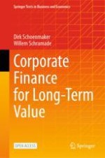
Finally, we put rFV, rSV, and rEV together to obtain the cost of integrated capital, rIV, which is the return on integrated assets that is demanded by the company’s stakeholders on aggregate. Interestingly, rIV gives an indication of the overall risk of the company, which can differ substantially from the risk picture that emerges from a purely financial perspective, even if that financial perspective is taken on an ESG integrated basis. Financial markets correct unsustainable activities to only a limited degree. An integrated perspective is needed to capture the full risk of not operating sustainably. And it might be the precursor of future financial risk. See Fig. 13.1 for a chapter overview.
A chart presents the overview of Chapter 13.1, which includes the cost of financial capital, F V. Chapter 13.2, Integrating sustainability into the cost of financial capital, F V plus E and S. Chapter 13.3, the cost of social and environmental capital S V and E V. Chapter 13.4, the cost of integrated capital.
Fig. 13.1
Chapter overview
×
Learning Objectives
After you have studied this chapter, you should be able to:
calculate the cost of capital for equity, debt, social capital, environmental capital, and integrated capital
explain the drivers of the various cost of capital measures
relate the costs of the various types of capital to each other
apply the appropriate cost of capital measure for valuing a company or project
appraise the cost of integrated capital and its implications
13.1 The Cost of Financial Capital
When evaluating investments using a DCF analysis (see Chaps. 4–7), managers and investors need an estimate of the cost of capital for those investments to discount future cash flows. What is the minimum return that is needed given the risk profile of the investment? For shareholders, this is the cost of equity; for bondholders, the cost of debt; and for corporate managers, it is the project cost of capital.
Advertisement
13.1.1 Cost of Equity Capital
The cost of equity is the return a company theoretically pays to its shareholders, to compensate for the risk they undertake by investing their capital. That compensation depends not only on the risk of the specific investment, but also on the pricing of risk on similar and other investments, the degree of risk aversion, and the supply and demand of capital. This is not exact science, but an approximation is given by the capital asset pricing model (CAPM, see Sect. 12.4), which gives the cost of equity capital ri of security (company) i given its systematic risk measured by beta βi:
With the risk premium for security i being: βi ∙ (E[rMKT] − rf);
And the market risk premium is: (E[rMKT] − rf).
Making assumptions or estimates on the parameters of the above formulae allows us to draw the security market line for security i in Fig. 13.2.
A plot of the cost of equity over beta. The upward slope from 2% on the y-axis indicates a security market line that reaches 10% at 2. The arrow at the origin of the line represents the risk-free rate. Horizontal and vertical lines from 6% and 1 from the axes intersect at the slope.
Fig. 13.2
The security market line
×
In Fig. 13.2, the risk-free rate is 2%, the expected market return is 6%, and hence the market risk premium is 6–2% = 4%. At a beta of 0, the cost of equity equals the risk-free rate, that is 2%. The cost of equity rises proportionally with beta, hitting 6% (i.e. the expected market return) at a beta of 1, and rising well above that at betas above 1.
In practice it is quite difficult to establish the security market line, since the exercise is littered with empirical questions, such as: What is the market portfolio? What is the risk-free rate? What is the beta of a specific security? What is the horizon of the expected return? To what extent are historical data representative of the future?
Estimating the Market Risk Premium
The market risk premium in Eq. 13.1 is defined as the expected market return E[rMkt] minus the risk-free rate rf. The risk-free rate is derived from the government yield curve, which provides the safest asset in a country (see Chap. 4). The maturity choice of the risk-free rate should match the maturity of the cash flows. For long-term assets, such as stocks, the 10-year or 30-year government bond yield provides a good proxy for the risk-free rate. Figure 4.8 shows that the risk-free rate on long-term US government bonds was about 3.5% and about 2% on long-term German government bonds (the benchmark for euro-area stocks) at the time of writing in late 2022.
The estimation of the market risk premium is more demanding. Chapter 12 highlights that the historical risk premium can only be estimated over a long period because markets fluctuate. Table 13.1 provides evidence for the US stock market (which makes up about 65% of the world stock market), Europe (which makes up about 20% of the world stock market), and the world market. Table 13.1 shows that the observed risk premium has declined over time. The evidence suggests a risk premium over 1-year government bonds of 3.5–6.5% and a risk premium over 10-year government bonds of 3–5%.
A company’s beta is a measure of the company’s stock price volatility relative to the market’s volatility. Historical betas can be estimated using linear regression analysis on historical returns against the relevant index (see Box 12.3 on leading market indices). For the market portfolio, typically a well-known index is chosen, such as the S&P500 or the MSCI World Index. Let’s apply this to two large listed companies with comparable activities: Nike ($196 billion market cap) and Adidas (€38 billion market cap), as of April 2022. Betas are often calculated on a 5-year monthly basis (5*12 = 60 observations) or on a 2-year weekly basis (2*52 = 104 observations), but one can use different frequencies and windows as well. This can give quite different results, as measuring at shorter frequencies leads to higher volatility. Taleb (2007) argues that volatility measured at short frequencies (e.g. 1 day or 1 week) contains a lot of random noise and he therefore recommends focusing on longer frequencies. Table 13.2 gives 2-year, 5-year, and 10-year betas, against both a home country index and a world index, first on a monthly and then on a weekly basis, for Nike and Adidas.
Table 13.2
Nike & Adidas betas
Monthly beta
Nike
Adidas
vs S&P500
vs MSCI World
vs DAX30
vs MSCI World
2-year
0.80
0.80
0.81
0.94
5-year
0.92
0.92
0.69
0.81
10-year
0.77
0.73
0.72
0.77
Average
0.83
0.82
0.74
0.84
Weekly beta
Nike
Adidas
vs S&P500
vs MSCI World
vs DAX30
vs MSCI World
2-year
1.16
1.20
1.22
1.17
5-year
1.05
1.12
1.07
1.00
10-year
1.01
1.00
0.94
1.02
Average
1.07
1.11
1.08
1.06
Note: All betas are calculated using data series ending in December 2021
As expected, the betas of both companies are quite similar to each other, since they are in the same industry. However, whereas the monthly betas of both companies are well under one (0.81 on average), their weekly betas are 34% higher (1.08 on average). In addition, there is also quite a difference for Adidas between the world index and the home country index (DAX30), which is partly a result of Nike’s home index (S&P500) being much bigger in the world index than the DAX.
The above numbers show that historical betas can differ significantly, depending on the way they are calculated in terms of frequency, window, and index used. But perhaps a more fundamental problem is that beta is meant to be forward-looking. Hence, historical betas may not be representative since a company’s systematic risk can change over time. See Chap. 12 for a discussion of forward-looking risk. The methods discussed there can be used to adjust historical betas.
Another problem is that betas can only be calculated for companies with sufficient historical pricing data, i.e. only for companies that have been listed for a while, not for unlisted (private) or recently-listed companies. In such a case, however, one can make an estimate of beta by looking at betas of comparable companies. Suppose a Norwegian salmon harvesting company is on the verge of doing an IPO (an initial public offering, i.e. listing of its stock on a stock exchange; see Chap. 16). The investment bankers helping on the IPO, as well as the investors who are interested in participating in the IPO, can then estimate the company’s beta by considering the betas of other Norwegian salmon harvesters. Table 13.3 gives an overview of those betas and nicely illustrates why that’s not a completely trivial exercise.
Table 13.3
Industry betas for Norwegian salmon harvesting
vs MSCI World
5-year monthly beta
2-year weekly beta
Average beta
Bakkafrost
0.41
0.48
0.45
SalMar
0.31
0.21
0.26
Mowi
0.70
0.46
0.58
Leroy Seafood
0.55
0.58
0.57
Austevoll Seafood
0.64
0.59
0.62
Grieg Seafood
0.62
0.74
0.68
Norway Royal Salmon
0.00
0.34
0.17
Average
0.46
0.48
0.47
Median
0.55
0.48
0.57
Average (without Royal)
0.54
0.51
0.52
First, betas can be measured in several ways, as discussed. Table 13.3 gives two of them: 5-year monthly betas (5*12 = 60 observations) and 2-year weekly betas (2*52 = 104 observations). So, they differ both in frequency and in time period. That is important since betas can change over time.
Second, how to aggregate the observations: do you take the average or the median of the betas? And do you include or exclude outliers? In the above example, Norway Royal Salmon has a striking 5-year monthly beta of 0.00, and while its 2-year weekly beta looks more normal, it is still significantly lower than the betas of its peers. Taking the 5-year monthly beta, we find an average beta of 0.54 (excluding Norway Royal Salmon) which is close to the median of 0.55. Even after making these adjustments, one can still question if such a low beta is the right estimate going forward.
Example 13.1 shows how one can calculate the cost of equity capital for the Norwegian salmon farmer, using industry betas.
Example 13.1 Calculating the Cost of Equity Capital
Problem
Suppose the risk-free rate is 2% and the market risk premium is 4%. What is the cost of equity capital for a Norwegian salmon farmer?
Solution
First, we have to make a choice for the maturity of the estimated betas (monthly vs weekly). As longer-term betas are more stable, we choose the 5-year monthly beta from Table 13.3. Next, we take the industry average without the outlier Norway Royal Salmon. This gives us a beta of 0.54.
We can calculate the expected return by taking the cost of equity capital Eq. 13.1:
As explained, the low beta for the Norwegian salmon industry gives us a rather low cost of equity capital of 4.2%.
13.1.2 Cost of Debt Capital
The cost of debt can be calculated in a similar way as the cost of equity, by estimating debt betas using CAPM. However, that is hard given the infrequent trading of most public debt. Moreover, the risk of default (and thus the debt beta) is very low for investment-grade bonds, as shown in Table 13.4. The cost of debt is more commonly calculated using credit ratings, as described in Chap. 8. Following Eq. 8.8, the cost of debt rD can be calculated as follows:
Table 13.4
Default rates and debt betas by credit rating
A table with two sections has 5 columns and 9 rows. The column headers are rating agency, Moody's, S and P's and Fitch, long-term average default, and debt betas. The subheaders of the first section are type of bonds and investment grade bonds and in the second section type of bonds and high yield bonds.
Source: S&P Global Ratings (2020a) for long-term default rates (1981–2019 average) and Berk and DeMarzo (2020) for debt betas
where PD is the probability of default, y is the yield (promised interest), and LGD the loss given default (the fraction of the principal and interest lost in case of default). While the yield y can be observed in the market, we need estimates for PD and LGD. Using Box 8.1 from Chap. 8, Table 13.4 shows that the default rates PD and debt betas βD are quite low for investment-grade bonds, but can be much higher for junk bonds. The extremes on both sides are interesting. On the safe side, AAA, AA, and A rated bonds have extremely low credit risk with default rates at 0.00, 0.02, and 0.05%, respectively, and the debt beta is below 0.05. A company’s debt beta measures the volatility of the company’s debt relative to the market’s volatility. On the risky side, default rates for CCC, CC, and C rated bonds increase to over 25% and only for CCC rated bonds can a reliable beta of 0.31 be estimated. So, it often does not make sense to use debt betas for relatively safe bonds, since they are very low and difficult to estimate precisely. Finally, the long-term average loss given default rate LGD, the last variable of Eq. 13.2 to estimated, is 60% for bonds (S&P Global Ratings, 2020b).
Example 13.2 shows how we can calculate the cost of debt capital for a salmon farmer.
Example 13.2 Calculating the Cost of Debt Capital
Problem
The Norwegian salmon farmer, SalMar, has a rating of BBB and a yield of 3.22% in June 2022. The loss given default is 60%. What is SalMar’s cost of debt capital?
Solution
Using Table 13.4, a BBB rating implies a probability of default (PD) of 0.16%. The loss given default (LGD) is 60%. And the yield is 3.22%.
We can calculate the cost of debt capital using Eq. 13.2:
Debt and equity are just components of the company’s overall capital. How can we calculate the company’s cost of capital? Table 13.5 provides a balance sheet for company X, based on market values.
Table 13.5
Market-value balance sheet, company X
Value
Discounted at
Value
Discounted at
Assets
100
?%
Debt
D = 40
2.5%
Equity
E = 60
10%
Enterprise value
V = 100
?%
Enterprise value
V = 100
?%
The sum of debt D and equity E provides the company’s overall value (the right side of Table 13.5). In Chap. 9, we introduced enterprise value V as the market value of the company’s underlying business (using its assets) before financing by equity and debt (the left side of Table 13.5). To balance both sides of the balance sheet, the company’s overall value (based on equity and debt) should match the company’s enterprise value (based on assets). We can thus derive the simplified equation for enterprise value V as follows:
$$ \mathrm{Enterprise}\ \mathrm{value}:V=E+D $$
(13.3)
Likewise, the cost of debt and the cost of equity are components of the overall cost of capital rU, which is also known as the weighted average cost of capital (WACC):
The calculation of WACC seems straightforward since it is the weighted average of the cost of equity capital rE and the cost of debt capital rD. In our simple example of company X in Table 13.5, the WACC is 0.6 ∗ 10 % + 0.4 ∗ 2.5 % = 7%.
However, it should be noted that the presence (and weight) of debt in the capital structure affects the cost of equity. Chapter 15 (capital structure) shows the effect of leverage on the cost of equity capital. Another aspect is the presence of corporate tax. As interest expenses can be deducted from taxable income, the after-tax interest rate is the relevant indicator for a company’s net cost of debt capital: rD ∙ (1 − τC), whereby τC is the company’s tax rate. The tax-adjusted WACC formula becomes then:
The tax savings reduce the cost of capital of a levered company in comparison with the cost of capital of an unlevered company rU. Combining Eqs. 13.4 and 13.5, we get:
Assuming a corporate tax rate of 20%, the after-tax WACC of company X is 0.6 ∗ 10 % + 0.4 ∗ 2.5 % ∗ (1 − 0.20) = 6.8%. The after-tax WACC is 0.2% lower than the WACC of 7.0%. We can check this calculation by calculating the tax savings (the second term in Eq. 13.6): \( \frac{D}{V}\bullet {r}_D\bullet {\tau}_C=0.4\ast 2.5\%\ast 20\%=0.2\% \). The role of corporate tax and related tax savings is further discussed in Chap. 15 on capital structure.
Examples 13.3 and 13.4 show how you can calculate the WACC for a company.
Example 13.3 Calculating the WACC
Problem
Company Y has a cost of equity capital of 8% and a cost of debt capital of 3%. The company’s market capitalisation is € 200 million and its outstanding debt € 70 million. The corporate tax rate is 25%. What is the unlevered cost of capital and what is the after-tax WACC for company Y?
Solution
Combining equity (market cap) and debt, we obtain company’s Y value at € 270 million. We can now calculate the unlevered cost of capital rU using Eq. 13.4:
The after-tax WACC is lower than the pre-tax WACC (the unlevered cost of capital) due to tax savings on the interest payments. To check: \( \frac{D}{V}\bullet {r}_D\bullet {\tau}_C=\frac{70}{270}\ast 3\%\ast 25\%=0.2\% \).
Example 13.4 Calculating SalMar’s WACC
Problem
We would like to calculate the WACC of our Norwegian salmon farmer, SalMar. Suppose the risk-free rate is 2% and the market risk premium is 4%. SalMar’s beta is 0.31 (Table 13.3) and its cost of debt capital is 3.12% (Example 13.2). Next, SalMar’s equity is NOK 50.6 billion and its debt is NOK 12.6 billion. The Norwegian corporate tax rate is 22%.
What is the cost of equity and the pre-tax and after-tax WACC of SalMar?
Solution
The first step is to calculate the cost of equity using Eq. 13.1:
The pre-tax WACC is 3.22% and the after-tax WACC 3.08%. SalMar’s low beta of 0.31 and low leverage of 19.9% \( \left(=\frac{D}{V}=\frac{12.6}{63.2}\right) \) give it a very low cost of capital.
13.1.4 Project Cost of Capital
Company betas reflect the market risk of the average project in a company. Project risk can deviate substantially from company risk. For example, when a pharmaceutical company wants to invest in a new headquarters building, the beta of the pharmaceutical industry is not very helpful. It is better to use the beta of commercial real estate to determine the project’s cost of capital. So, it is important to identify companies or sectors comparable to the project.
The observed company betas are related to equity βE. These company betas are levered, i.e. they reflect the leverage of the companies involved. But unlevered ones are needed, which reflect the beta of a company’s total assets (see Fig. 13.3). The asset beta, or unlevered beta βU, is calculated as follows:
A chart outlines the consecutive stages involved in calculating the project beta. It starts with determining the levered equity beta, then the unlevered asset beta, and finally the project beta.
Most unlevered (asset) betas are lower than levered (equity) betas, reflecting the lower risk of the underlying assets before levering up. Going back to our Norwegian salmon farmer, Table 13.6 shows the levered betas (columns 2 and 3) taken from the market (see Table 13.3) and the unlevered betas (columns 5 and 6) calculated with Eq. 13.7. The bottom row of Table 13.6, which excludes the outlier Norway Royal Salmon, provides the industry betas for Norwegian salmon harvesting. For ease of exposition, we assume that the beta of debt is zero in our calculations. Debt betas are usually very low, as shown earlier in Table 13.4.
Table 13.6
Industry betas for Norwegian salmon harvesting
vs MSCI World
5-year monthly beta
2-year weekly beta
E/(E + D)
Unlevered 5-year monthly beta
Unlevered 2-year weekly beta
Average
Bakkafrost
0.41
0.48
0.77
0.32
0.37
0.34
SalMar
0.31
0.21
0.67
0.21
0.14
0.17
Mowi
0.70
0.46
0.63
0.44
0.29
0.36
Leroy Seafood
0.55
0.58
0.71
0.39
0.41
0.40
Austevoll Seafood
0.64
0.59
0.55
0.35
0.32
0.34
Grieg Seafood
0.62
0.74
0.64
0.39
0.47
0.43
Norway Royal Salmon
0.00
0.34
0.58
0.00
0.20
0.10
Average
0.46
0.49
0.65
0.30
0.31
0.31
Median
0.55
0.48
0.64
0.35
0.32
0.34
Average (without Royal)
0.54
0.51
0.66
0.35
0.33
0.34
Figure 13.3 shows the steps from an observed (levered) equity beta to an unlevered asset beta. The final step is to select the relevant asset beta for the project. Figure 13.4 provides an overview of industry asset betas. The total market asset beta is 0.93. High risk industries are semiconductors (asset beta of 1.49), information services (1.16), oil and gas production and exploration (1.13), and chemicals (1.06). By contrast, stable industries are utilities (0.50), real estate (0.58), and telecom (0.65). Example 13.5 shows how we can calculate the pharmaceutical company’s cost of capital for its headquarters.
A bar graph plots the industry asset betas. The total market value is 0.93 which is indicated by an arrow. Other betas include steel, technology, retail, beverage, broadcasting, and so on.
Fig. 13.4
Industry asset betas (2022). Source: Data from Damodaran (2022). Note: Assets betas are based on 2-year and 5-year weekly betas for global companies. The total market asset beta (0.93) is without financials
×
Example 13.5 Calculating the Headquarters’ Project Cost of Capital
Problem
Pharma company X wants to build a new headquarters. It is fully financed with equity. The risk-free rate is 3% and the market risk premium is 4%. What is the project’s cost of capital?
Solution
As explained, we should take the real estate asset beta of 0.58 instead of the pharma beta of 0.97, which are both taken from Fig. 13.4. As the headquarters is fully equity financed, the unlevered or asset beta can be used to calculate the project’s cost of capital. Using Eqs. 13.4 and 13.1, we can calculate the project’s cost of capital:
The project’s cost of capital of 5.3% is lower than the pharma company’s cost of capital of 6.9% = 3% + 0.97*4%. So, the cost of capital better reflects the risk of the project when selecting the appropriate asset beta for the building project.
13.2 Integrating Sustainability into the Cost of Financial Capital
Let’s now explore how S and E risks could affect the cost of financial capital. There is empirical evidence that S and E affect the cost of equity and the cost of debt. For example, companies with better sustainability scores tend to have cheaper financing (El Ghoul et al., 2011; Albuquerque et al., 2019) and better access to finance (Cheng et al., 2014). These effects can be expressed and estimated in an adjusted cost of equity capital.
13.2.1 Adjusted Cost of Equity Capital
The factor behind a lower cost of equity capital is lower systematic risk. Companies with better sustainability performance have lower betas for social risk \( {\beta}_i^{SF} \)and/or environmental risk \( {\beta}_i^{SF} \). From Chap. 12, we reproduce the adjusted cost of equity capital Eq. (12.16):
+ \( {\beta}_i^{SF} \) x social risk premium + \( {\beta}_i^{EF} \) x environmental risk premium
As social and environmental risks have only recently been considered as relevant for stock prices, there are no long-term estimates for the social and environmental risk premium yet, unlike for the market risk premium. Chapter 12 provides emerging evidence on the social and environmental risk premium. Table 13.7 shows that the social risk premium is in the range of 1.0–1.5%, while the environmental risk premium is 1.9%.
The challenge is to estimate company betas for social and environmental risk. We cannot derive historical betas like those for market risk, as there is no reliable history of the social and environmental index against which we can regress historical company returns. For the estimation of company exposure to social and environmental risks, we can use several approaches. The most comprehensive approach is a value-based approach using our estimates for SV and EV, based on material social and environmental factors. Negative values for SV and EV indicate that a company causes social and environmental problems. So, it is exposed to social and environmental risks, which implies a positive beta \( {\beta}_i^{SF},{\beta}_i^{EF}>0 \). By contrast, positive values for SV and EV show that a company contributes to solving social and environmental challenges, which implies a negative beta \( {\beta}_i^{SF},{\beta}_i^{EF}<0 \). SV and EV thus are negatively related to the social and environmental betas. But how can we estimate the precise size of the social and environmental betas? A pragmatic method to gauge the effect of a company’s social and environmental risks on its financial risk profile is to relate SV and EV to FV. We can thus derive a proxy for the factor betas:
The calculation of the factor betas is straightforward, once we know a company’s social, environmental, and financial value (see Chap. 5). For example, an oil company with a large negative EV (due to large scope 3 carbon emissions) relative to its FV faces a high environmental beta. A pharmaceutical company that is developing drugs that can save lives has a positive SV and thus a negative social beta.
Of course, when data are not available to perform a complete calculation of SV and EV, you can make ad hoc assessments of the factor betas according to S and E exposures. For example, in the abovementioned salmon harvesting example, one could argue that health and climate concerns might lower social and environmental betas in the near future (since salmon is healthier than beef and pork, at lower carbon footprints), whereas a potential taboo on eating animals would increase its social beta in the longer run. Key is to include all material social and environmental factors in your assessment.
Another, albeit more debatable (see below), approach to calculate factor betas is using a company’s ESG ratings, which have an environmental, social, and governance pillar. Referring back to Sect. 12.5, remember that our environmental risk premium is based on a broad environmental score, across 13 environmental issues related to climate change, natural resources, pollution, and waste. So, we need broad environmental and social scores for companies. Next, the social and environmental factor portfolios are constructed as bad (the lowest third) minus the good (the top third), which represents a wide difference in social and environmental performance between companies. Companies with low scores have high betas, while companies with high scores have low (or even negative) betas. This negative relationship might be counterintuitive, but is correct. Low S and E scores indicate a poor performance on S and E factors and thus a high exposure to social and environmental risks, which is measured by the social and environmental beta, respectively.
Given the wide availability of ESG ratings, this ESG approach is tempting, but it has severe limitations. First, this approach only works with absolute scores. So, all companies with severe environmental problems get a low environmental score. However, some ESG ratings methods, like the best-in-class method, use relative scores. Best-in-class assigns high scores to the leaders within an industry (regardless of the industry environmental profile). The best oil company (i.e., the oil company with the least amount of carbon emissions) would then get a high score, as best-in-class. But this oil company will still have large carbon emissions (suggesting a low absolute score). Second, there are severe shortcomings with ESG ratings, as highlighted in Box 14.3 in Chap. 14.
Example 13.6 provides an example of calculating the adjusted cost of equity capital for a chemical company. As can be expected, the chemical company’s adjusted equity cost is higher due to pollution and carbon emissions. Estimating the adjusted cost of equity capital is work in progress, as S and E risks are only recently included in empirical estimations and not yet available for many companies. The adaptive markets hypothesis suggests that the quality of the estimations and the number of companies covered may increase over time when more data becomes available and more analysts pay attention. In the absence of hard data, heuristics may be superior. In practice, equity analysts tend to make direct adjustment in the cost of equity capital, rather than via beta, as for example shown in case studies of the Principles for Responsible Investing (PRI, 2018).
Example 13.6 Calculating the Adjusted Cost of Equity Capital
Problem
An American chemical company has a market beta of 1.1 and an enterprise value of $50 million. Its environmental value is −$60 million and its social value −$10 million. The risk-free rate is 3% and the market risk premium is 4%. What is the chemical company’s cost of equity capital? And what is the chemical’s company adjusted cost of equity capital? Please use the value-based method to calculate the adjusted cost of equity capital.
Solution
Let’s start with the cost of equity capital, using Eq. 13.1:
So, the chemical company has a cost of equity capital of 7.4%. The provided data indicate that the chemical company has major environmental problems and minor social problems. Let’s see to which adjustments this leads in the cost of equity capital. Using the value-based method, we derive the social and environmental beta as follows, using Eq. 13.9:
Next, we can take the social and environmental risk premiums from Table 13.7. We can now insert these betas and risk premiums in the adjusted cost of equity capital (Eq. 13.8):
The value-based method, which includes social and environmental risks, leads to a substantially higher adjusted cost of equity capital of 9.9% than the cost of equity capital of 7.4%. This higher adjusted cost of equity capital reflects the social and environmental risks of the chemical company.
13.2.2 Adjusted Cost of Debt Capital
There is also evidence that sustainability concerns lead to higher cost of debt capital (Chava, 2014). Following Eq. 13.2, the cost of debt rD is calculated as follows:
Sustainability risks can increase the probability of default PD, which the debt provider translates into a higher contractual interest rate y. Remember that the yield y has to cover expected credit losses (related to PD) as well as a credit risk premium (see Chap. 8). The adjusted cost of debt capital thus rises.
Banks offer sustainability-linked loans, whereby the interest rate is linked to an external ESG rating. Box 13.1 provides an example where ING bank links the interest rate on a loan facility for health technology company Philips to its sustainability performance and rating. If the rating goes up, the interest rate goes down and vice versa. Philips is thus incentivised to improve its sustainability, while ING reduces the risk of its loan.
Box 13.1 Sustainability-Linked Loan for Philips
In April 2017, the healthcare technology company Philips agreed an innovative first-of-its-kind €1bn loan facility with a consortium of banks that features an interest rate linked to the technology firm’s year-on-year sustainability performance. The nature of the loan facility means if Philips’ sustainability performance improves (as measured by Sustainalytics), the interest rate it has to pay goes down, and vice versa.
As part of the consortium of 16 banks offering the loan, ING Bank has conducted the credit risk assessment and acted as the sustainability coordinator for the loan. Philips’ sustainability performance has been assessed and benchmarked by Sustainalytics, an independent provider of ESG ratings.
ING indicated that the loan agreement with Philips was an additional way for the bank to support and reward clients seeking to become more sustainable. The loan facility follows Philips’ ‘Healthy People, Sustainable Planet’ programme, through which it is aiming to become ‘carbon-neutral’ throughout its global operations and source all of its electricity needs from renewable sources (SDG 12) and to improve the lives of 3 billion people a year by making the world healthier and more sustainable through innovation (SDG 3).
In a 2022 repeat transaction for Philips, ING again acted as sustainability coordinator, arranging a sustainability-linked loan with ambitious KPIs aligned with Philips’ sustainability goals for lives improved, lives improved in underserved communities, circular revenues, and operational carbon footprint.
The adjustment for sustainability risks is small for investment-grade debt (just a few basis points), as the credit risk on this debt is already very low anyway. Bigger adjustments to the cost of debt capital can be made for junk bonds, which are riskier. As the credit risk on junk bonds is more similar to equity risk, adjustments to the cost of debt capital can be made in a similar way, as shown above, for the adjusted equity risk of capital.
13.2.3 Adjusted WACC
The calculation of a company’s WACC remains the same (see Eqs. 13.4 and 13.5). Only the inputs of rE (ri from Eq. 13.8) and rD (from Eq. 13.10) into the WACC calculation change. Example 13.7 calculates the adjusted WACC of our chemical company.
Example 13.7 Calculating the Adjusted WACC
Problem
Our American chemical company, introduced in Example 13.6, has a market capitalisation of $40 million and a debt of $10 million. The cost of debt capital is 4%. What is the chemical’s company WACC? And what is the chemical’s company adjusted WACC?
Solution
The enterprise value of $50 million is financed by equity of $40 million and debt of $10 million. The low leverage indicates that the chemical’s company debt is relatively safe and thus investment grade. Using Eq. 13.4, we can calculate the WACC as follows:
As the chemical’s company cost of debt is investment grade, the adjustment for sustainability risks is small. So, there is no need to adjust the cost of debt. The adjusted cost of equity is 9.9% (see the value-based method in Example 13.6). The adjusted WACC becomes then:
The adjusted WACC is 2% higher than the WACC. This higher adjusted WACC reflects the chemical company’s environmental risk.
13.3 The Cost of Social and Environmental Capital
The previous section discussed the impact of S and E risks on the cost of financial capital, but S and E also have their own cost of capital. Given their nature, these tend to be much lower than a company’s cost of financial capital. The counterparty of companies’ SV and EV is the wider society, representing current and future generations. Low social discount rates imply that current and future generations are treated more or less equally. The flip side is that the valuation of liabilities on S and E tends to be quite high versus their value flows. They are an interesting expression of the claims that society and nature might have on companies.
From Chap. 12, we can take the social discount rate rs for discounting social and environmental capital (Eq. 12.20):
The first parameter δ reflects the time preference between current and future generations. Equal treatment of current and future generations gives us a time preference of zero: δ = 0. Next, the growth rate g is driven by growth in consumption. Given a diminishing marginal utility of consumption, the growth rate is multiplied by the elasticity of marginal utility of consumption η. The elasticity measures how utility changes with consumption. Finally, the risk parameter L reflects the extreme element of macroeconomic risk of rare disasters or society collapse. Table 13.8 reproduces the parameter estimates from Chap. 12.
Table 13.8 shows that the social discount rate is 2.2%. This social discount rate rs is applicable to the discounting of social capital rSV and environmental capital rEV. There is no differentiation across different forms of social and environmental capital. There is also no company-specific component, as the social discount rate reflects the cost from a societal perspective for using social and environmental capital, as discussed in Chap. 4.
A final question is about the correlation between company (or project) risk and growth risk. Given the low variance of consumption growth (Gollier, 2012), the correlation can be ignored for practical purposes. So, there is no need for company- or project-specific adjustments of the social discount rate.
What does such a low cost of social and environmental capital mean? A lower cost of capital leads to a higher present value of social and environmental flows (positive or negative) than the present value of financial flows with a higher cost of financial capital. Let’s illustrate this point with two examples. The first is a medtech company that produces medical equipment that helps recovering patients in extending their life (see Table 13.9). Assuming constant flows over time, Table 13.9 provides the annual cash flows and social flows. The medtech has annual cash flows of € 450 million, while the annual social flows are €150 million (based on 2000 lives extended at €75,000 per quality life year). The annual financial flows are three times the annual social flows. But discounting changes the picture. The present value of the annual cash flows is \( PV=\frac{CF}{r}=\frac{450}{0.066}=\mathrm{6,818} \) million and the present value of the annual social flows is \( \frac{150}{0.022}=\mathrm{6,818} \) million. These present values are equal! As the cost of social capital (2.2%) is three times smaller than the cost of financial capital (6.6%), the present value of €1 of social flows is three times larger than the present value of €1 of financial flows. So, the annual social flows translate into a relatively large social asset. For the medtech company, this means that its total (or integrated) value is for 50% determined by its financial flows and 50% by its social flows.
Table 13.9
Financial and social value of a medtech company
Medtech company
Value in EUR millions
Financial flows
Annual cash flows (in EUR millions)
450
Discount factor
6.6%
Financial value (PV in EUR millions)
6818
Social flows
Quality life years extended annually
2000
Quality life year in EUR
75,000
Annual social flows (in EUR millions)
150
Discount factor
2.2%
Social value (PV in EUR millions)
6818
Company value (in EUR millions)
13,636
The second example in Table 13.10 concerns an oil company, which sells oil at a net profit but is also responsible for the resulting carbon emissions from consumers’ use of the oil. Annual cash flows amount to €800 million. The annual carbon emissions attributed to the oil company is 1.8 million tonnes of CO2. At a shadow price of €200 per tonne, these annual carbon emissions translate into negative annual environmental flows of €360 million. This is slightly less than half of the annual financial flow. Assuming no social flows, the company’s annual total flows are € 440 (=800–360) million. But when we discount the two flows at their respective costs of capital, the picture changes dramatically. The financial value is €12,121 million (the continuous €800 million cash flow discounted at 6.6%), while the environmental value is € −16,364 million (the continuous negative €360 million environmental flow discounted at 2.2%). The annual carbon emissions turn into a very large negative environmental value. This puts the company’s value in negative territory (€ −4242 million).
Table 13.10
Financial and environmental value of an oil company
Oil company
Value in EUR millions
Financial flows
Annual cash flows (in EUR millions)
800
Discount factor
6.6%
Financial value (PV in EUR millions)
12,121
Environmental flows
Carbon emissions (thousands of tonnes CO2)
1800
Shadow price of emissions, EUR/tonne
200
Annual environmental flows (in EUR millions)
−360
Discount factor
2.2%
Environmental value (PV in EUR millions)
−16,364
Company value (in EUR millions)
−4242
These two company examples show that a low social discount rate can turn positive (negative) social and environmental flows into relatively large social and environmental assets (liabilities). Whereas financial discounting reduces the value of future cash flows substantially, social and environmental discounting does that to a lesser extent.
13.4 The Cost of Integrated Capital
In the previous sections, we considered \( {r}_i^{FV} \) (which is the adjusted WACC), rSV and rEV separately, as well as their drivers. We now put them together in the cost of integrated capital \( {r}_i^{IV} \) (Eq. 12.21), which is the return demanded on all types of capital combined.
An interesting exercise is to see what happens to \( {r}_i^{IV} \), when we keep FV and SV constant but let EV rise. In other words, what is the impact on the company’s cost of integrated capital when its environmental profile improves from −50 to +50? Table 13.11 shows our simulation. The starting position is: FV = 100, SV = 0, and EV = − 50. As we are only interested in the impact of changing EV, we put SV at zero. Next, the cost of the capitals is: \( {r}_i^{FV}=6.0\% \), rSV = 2.2%, and rEV = 2.2%. While keeping FV constant at 100, rIV moves from 9.8% when EV is −50 to 4.7% when EV is 50 in Table 13.11.
Table 13.11
Simulation of the cost of integrated capital
FV
SV
EV
IV
FV/IV
SV/IV
EV/IV
rFV
rSV
rEV
rIV
100
0
−50
50
2.0
0.0
−1.0
6.0%
2.2%
2.2%
9.8%
100
0
−40
60
1.7
0.0
−0.7
6.0%
2.2%
2.2%
8.5%
100
0
−30
70
1.4
0.0
−0.4
6.0%
2.2%
2.2%
7.6%
100
0
−20
80
1.3
0.0
−0.3
6.0%
2.2%
2.2%
7.0%
100
0
−10
90
1.1
0.0
−0.1
6.0%
2.2%
2.2%
6.4%
100
0
0
100
1.0
0.0
0.0
6.0%
2.2%
2.2%
6.0%
100
0
10
110
0.9
0.0
0.1
6.0%
2.2%
2.2%
5.7%
100
0
20
120
0.8
0.0
0.2
6.0%
2.2%
2.2%
5.4%
100
0
30
130
0.8
0.0
0.2
6.0%
2.2%
2.2%
5.1%
100
0
40
140
0.7
0.0
0.3
6.0%
2.2%
2.2%
4.9%
100
0
50
150
0.7
0.0
0.3
6.0%
2.2%
2.2%
4.7%
This table calculates the cost of integrated capital \( {r}_i^{IV} \). The first three columns provide the three dimensions, which can be added up to IV. Columns 5–7 calculate the weight of the value dimensions. Please note that these weights add up to 1, as required. The final columns provide the costs of capital, whereby \( {r}_i^{IV} \) is calculated as a weighted average of the cost of financial, social, and environmental capital
Figure 13.5 shows the declining trend graphically. The orange midpoint reflects the cost of financial capital of 6%. To the left are E liabilities EV < 0 which increase the cost of integrated capital. And to the right are E assets EV > 0 which reduce the cost of integrated capital.
A graph plots the cost of integrated capital. A downward slope declines from 9.8% to 4.6% between negative 50 and 50 E V. Horizontal and vertical lines from 6% and 0 from the y and x axis intersect at the slope. The left and right arrows to the left and right of 0 represent E liabilities and E assets, respectively.
Fig. 13.5
Cost of integrated capital
×
How should we interpret these results? The driving force behind the cost of integrated capital is the fact that the cost of financial capital is higher than the cost of social and environmental capital. The result is that the cost of integrated capital declines with higher amounts of positive social and environmental capital and rises when social and environmental capital fall and go negative. That follows directly from the weighted average formula in Eq. 13.12.
But what does it mean in economic terms? A company with environmental (or social) liabilities has a higher risk profile, reflected in a cost of integrated capital that exceeds its cost of financial capital. The company is basically taking a bet on the future, assuming that it can continue its business model with negative social and environmental externalities. But the company may have to pay for these externalities (i.e., internalisation) or, even worse, new regulations may forbid the company to draw down society’s social and environmental capital. The higher cost of integrated capital reflects this risk. By contrast, a company with environmental (or social) assets has a lower risk profile and thus a lower cost of integrated capital, as it offers solutions. When internalisation takes place, that company has a competitive advantage with a future-proof business model (see Chap. 2). The risk to the company’s business model is relatively low (i.e. the chance of maintaining the going concern is high), which is reflected in a low cost of integrated capital.
13.4.1 Adjusted Cost of Capital
Our simulation exercise was executed in a static way with constant cost of capital components: rFV = 6.0%, rSV = 2.2% and rEV = 2.2%. To what extent do the associated risks affect each other? The easy part is that the cost of social and environmental capital rSV and rEV remains constant, as explained in Sect. 13.3. But the adjusted cost of financial capital rFV rises with increasing social and environmental risks (proxied by negative values for SV and EV in Sect. 13.2). So, if anything, the dispersion in the cost of integrated capital widens in a dynamic simulation. The final columns of Table 13.12 compare the results of the dynamic and static rIV. Table 13.12 highlights that social and environmental factors influence the adjusted cost of financial capital rFV in a limited way (ranging from 5 to 7% in our example), while the cost of integrated capital rIV varies from 4 to 12%. Figure 13.6 shows the dynamic cost of integrated capital. The orange focal point of 6% at EV = 0 in Fig. 13.6 is the same as in Fig. 13.5, but the line is steeper than in Fig. 13.5: a higher dynamic cost of integrated capital at negative values of EV and a lower dynamic cost of integrated capital at positive values of EV.
Table 13.12
Dynamic simulation of cost of integrated capital
FV
SV
EV
IV
βSF
βEF
rFV
rSV
rEV
dynamicrIV
staticrIV
100
0
−50
50
0
0.5
7.0%
2.2%
2.2%
11.7%
9.8%
100
0
−40
60
0
0.4
6.8%
2.2%
2.2%
9.8%
8.5%
100
0
−30
70
0
0.3
6.6%
2.2%
2.2%
8.4%
7.6%
100
0
−20
80
0
0.2
6.4%
2.2%
2.2%
7.4%
7.0%
100
0
−10
90
0
0.1
6.2%
2.2%
2.2%
6.6%
6.4%
100
0
0
100
0
0
6.0%
2.2%
2.2%
6.0%
6.0%
100
0
10
110
0
−0.1
5.8%
2.2%
2.2%
5.5%
5.7%
100
0
20
120
0
−0.2
5.6%
2.2%
2.2%
5.1%
5.4%
100
0
30
130
0
−0.3
5.4%
2.2%
2.2%
4.7%
5.1%
100
0
40
140
0
−0.4
5.2%
2.2%
2.2%
4.4%
4.9%
100
0
50
150
0
−0.5
5.1%
2.2%
2.2%
4.1%
4.7%
This table calculates a dynamic cost of financial capital \( {r}_i^{FV} \) by adding the social and environmental risk premium. We use Eq. (13.8): \( {r}_i={r}_f+{\beta}_i^{MKT}\bullet {RP}_{MKT}+{\beta}_i^{SF}\bullet {RP}_{SF}+{\beta}_i^{EF}\bullet {RP}_{EF} \) and assume full equity financing, a risk-free rate of 2%, a market beta of 1, a market risk premium of 4%, a social risk premium of 1.25%, and an environmental risk premium of 1.9%. The factor betas are calculated with Eq. (13.9): \( {\beta}_i^{SF}=-\frac{SV}{FV}\kern0.5em \mathrm{and}\kern0.5em {\beta}_i^{EF}=-\frac{EV}{FV} \)
A graph illustrates the dynamic cost of integrated capital. The slope falls from 11.8% to 4%. Horizontal and vertical lines from the y and x axes intersect at the slope. The left and right arrows to the left and right of 0 represent E liabilities and E assets.
Fig. 13.6
Dynamic cost of integrated capital
×
An integrated perspective that includes social and environmental value in the calculations makes a big difference.
13.4.2 Inditex Case Study
We can now calculate the cost of financial capital and the cost of integrated capital for Inditex (see the case study in Chap. 11). Example 13.8 gives the basic data and shows the calculations. The starting point is Inditex’s cost of financial capital at 7.8%, as used in the Inditex case study in Chap. 11. Inditex’s net social and environmental liabilities of −$37 bn (= social assets of $146 bn—environmental liabilities of $183 bn) cause an uplift of the cost of capital. The first step is from 7.8 to 9.9% on the cost of financial capital, which is mainly caused by Inditex’s high sensitivity (beta) to the environmental risk premium. The second step is from 9.9 to 16.6% on the cost of integrated capital. The net social and environmental liabilities increase the cost of integrated capital, as shown in Fig. 13.6.
Inditex’s cost of integrated capital of 16.6% is far higher than its cost of financial capital, reflecting Inditex’s social liabilities (workers in the supply chain) and environmental liabilities (GHG emissions and other environmental damages). We cannot tell if that is higher compared to the overall market, since we do not (yet) have the integrated value data on other companies.
Example 13.8 Calculating the Cost of Financial and Integrated Capital for Inditex
Problem
From Chap. 11, we know that Inditex has a risk-free rate of 1.5%, a market risk premium of 5%, a beta of 1.21, and a credit risk premium of 1%. From Table 13.7 in this chapter, we know that the social risk premium is 1.25% and the environmental risk premium 1.9%.
For 2021, Inditex had an integrated value of €42 billion. Table 13.13 shows the components of the integrated value (taken from Table 11.18 in Chap. 11). In addition, Inditex had equity of €82 billion and a negative debt of −€3 billion (taken from Table 11.6; debt is negative due to Inditex’s large cash position).
Please calculate Inditex’s adjusted cost of financial capital and cost of integrated capital.
Solution
Cost of financial capital
Let’s first reproduce Inditex’s cost of financial capital. The cost of financial capital is the WACC based on the cost of equity and the cost of debt. Using Eq. 13.1, we get for the cost of equity rE = rf + βi ∙ (E[rMKT] − rf) = 1.5 % + 1.21 ∗ 5 % = 7.6%. Using Eq. 8.10, the cost of debt is rD = rf + CRP = 1.5 % + 1.0 % = 2.5%. Now we can calculate Inditex’s cost of financial capital: \( WACC=\frac{E}{V}\bullet {r}_E+\frac{D}{V}\bullet {r}_D=\frac{82}{79}\ast 7.6\%-\frac{3}{79}\ast 2.5\%=7.8\% \).
The next step is to calculate the adjusted cost of financial capital. Starting with the adjusted cost of equity component, we need to calculate the betas for social risk and for environmental risk using Eq. 13.9:
Please note that the positive social value of $283 bn and the negative social value of −$137 bn add up to SV of $146 bn. We use Eq. (13.8) for the adjusted cost of equity:
There is no change in Inditex’s cost of debt assumed—at higher debt levels, that might be an unrealistic assumption. Inditex’s adjusted cost of financial capital is \( WACC=\frac{E}{V}\bullet {r}_E+\frac{D}{V}\bullet {r}_D=\frac{82}{79}\ast 9.6\%-\frac{3}{79}\ast 2.5\%=9.9\% \). So Inditex’s adjusted cost of financial capital of 9.9% is 2.1% higher than the earlier calculated cost of financial capital of 7.8%.
Cost of integrated capital
We now have all the ingredients to calculate Inditex’s cost of integrated capital. Using Eq. 13.12, we get:
Inditex’s net social and environmental liabilities of −$37 bn (= social assets of $146 bn—environmental liabilities of $183 bn) cause an uplift of the cost of capital: from 7.8 to 9.9% on the cost of financial capital and from 9.9 to 16.6% on the cost of integrated capital.
13.4.3 Assets Versus Liabilities
Example 13.9 shows the impact of social and environmental liabilities versus assets for almost identical companies. The presence of liabilities puts a company at risk of increasing the cost of integrated capital. In capital structure terms, the company has higher leverage. By contrast, social and environmental assets improve a company’s risk profile (with lower leverage) reducing the cost of integrated capital. We explore the effect of leverage further in Chap. 15 on capital structure. Example 13.9 highlights that even modest differences in social and environmental flows can have a large impact on a company’s risk profile. The cost of integrated capital is thus a good indicator of a company’s future-proofness or transition preparedness, as discussed in Chap. 2.
Example 13.9 Calculating the Cost of Integrated Capital for Almost Identical Companies
Problem
Let’s compare two companies, A and B. They are identical from an FV perspective: both have annual FV flows of 6.4 and a cost of financial capital of 8%. However, company B is superior to company A on both annual SV flows (0.4 vs 0.2) and annual EV flows (0.2 vs −0.4). Both have a cost of social and environmental capital of 2.2%.
What is the integrated value and cost of integrated capital of both companies? Please explain the differences.
Solution
The first step is to transform the annual value flows into present value. We can use Eq. 4.6: \( PV=\frac{CF}{r} \). The table below shows the results:
Company A
Company B
Value flows
Cost of capital
Value
Value flows
Cost of capital
Value
FV
6.4
8.0%
80.0
6.4
8.0%
80.0
EV
−0.4
2.2%
−18.2
0.2
2.2%
9.1
SV
0.2
2.2%
9.1
0.4
2.2%
18.2
IV
6.2
70.9
7.0
107.3
While the value flows only differ by 13%, the company values differ by 51%. The low cost of social and environmental capital magnifies the differences in social and environmental value.
The second step is to calculate the cost of integrated capital. We can use Eq. 13.12: \( {r}_i^{IV}=\frac{FV}{IV}\bullet {r}_i^{FV}+\frac{SV}{IV}\bullet {r}^{SV}+\frac{EV}{IV}\bullet {r}^{EV} \). The table below shows the results:
Company A
Company B
Value
Value weight
Cost of capital
Weighted CoC
Value
Value weight
Cost of capital
Weighted CoC
FV
80.0
113%
8.0%
9.0%
80.0
75%
8.0%
6.0%
EV
−18.2
−26%
2.2%
−0.6%
9.1
8%
2.2%
0.4%
SV
9.1
13%
2.2%
0.3%
18.2
17%
2.2%
0.2%
IV
70.9
100%
8.7%
107.3
100%
6.5%
The value weights are calculated as: \( \frac{FV}{IV},\frac{SV}{IV},\mathrm{and}\ \frac{EV}{IV} \). The final column for each company calculates the cost of integrated capital as weighted cost of financial, social, and environmental capital. Company A’s cost of integrated capital of 8.7% is much (220 bps) higher than company B’s cost of integrated capital of 6.5%. It is also quite a bit (70 bps) higher than its own cost of financial capital, because of its negative environmental value flows. By contrast, company B has a cost of integrated capital that is much (150 bps) lower than its cost of financial capital—which will be the case for any company with positive SV and EV. In sum, company B has future-proofed its business model producing positive social and environmental flows.
13.5 Conclusions
This chapter investigates the company’s cost of capital. It starts with the cost of financial capital rFV, which is the required minimum return on financial capital that is used in investment decisions. One can apply rFV to specific types of financial capital and it is typically expressed in terms of the WACC (weighted average cost of capital) for the company’s overall cost of capital; the cost of equity rE; the cost of debt rD; or the project cost of capital. Subsequently, the impact of S (social) and E (environmental) risks on the cost of financial capital is considered. That is, to what extent do companies incur additional (or reduced) financial risk from their S and E exposures?
It then addresses the cost of social capital rSV and the cost of environmental capital rEV in their own right. Given their nature, these tend to be much lower than a company’s cost of financial capital. The flip side is that the valuation of assets and liabilities on E and S tends to be quite high versus their underlying value flows, as discounting with a low discount rate has a limited impact on value. They are an interesting expression of the claims that nature and society might have on companies.
Finally, rFV, rSV, and rEV are put together to obtain the cost of integrated capital, rIV, which is the return on integrated assets demanded by the company’s stakeholders. Interestingly, rIV gives an indication of the overall risk of the company, which can differ substantially from the risk picture that emerges from a purely financial or an ESG integrated perspective. Financial markets correct unsustainable activities only to a limited degree. An integrated perspective is needed to capture the full risk of not operating in a sustainable way.
Key Concepts Used in This Chapter
Adjusted cost of capital includes sustainability (social and environmental factors) in the cost of capital
Asset beta measures the beta (see below) for a company without leverage; it is also called the unlevered beta
Beta measures the sensitivity of a company’s stock price to general market movements (with reference to market, social or environmental risk)
Capital Asset Pricing Model (CAPM) is the main asset pricing model in finance explaining the relationship between risk and return
Cost of capital refers to the required return on an investment
Factor beta measures the sensitivity of a company’s stock price to specific factors (e.g., the social factor or environmental factor)
Factor portfolio is a portfolio with unit risk exposure to a particular risk factor (market, social or environmental risk) and no risk exposure to other factors
Financial discount rate or cost of financial capital is the discount rate used to discount financial capital.
Industry beta measures the asset beta (see above) for an industry
Integrated discount rate or cost of integrated capital is the discount rate used to discount integrated capital (or value)
Market index represents an entire stock market and thus tracks the market’s changes over time
Market portfolio refers to the portfolio which contains all available assets in a market
Risk refers to the variation of future returns
Risk-free asset is a safe asset, such as government bills or bonds
Risk premium refers the return on a risky asset, such as equities or real estate, minus the return on the risk-free asset,
Security market line plots the expected return against the risk (measured by the beta) of each stock
Social discount rate is the discount rate for social projects and can be used to discount social and environmental capital.
Systematic risk refers to market-wide risk that cannot be diversified in a portfolio
WACC (weighted average cost of capital) is the weighted average of equity capital and debt capital
Open Access This chapter is licensed under the terms of the Creative Commons Attribution 4.0 International License (http://creativecommons.org/licenses/by/4.0/), which permits use, sharing, adaptation, distribution and reproduction in any medium or format, as long as you give appropriate credit to the original author(s) and the source, provide a link to the Creative Commons license and indicate if changes were made.
The images or other third party material in this chapter are included in the chapter's Creative Commons license, unless indicated otherwise in a credit line to the material. If material is not included in the chapter's Creative Commons license and your intended use is not permitted by statutory regulation or exceeds the permitted use, you will need to obtain permission directly from the copyright holder.