This chapter examines methods to derive the equity value of publicly listed companies. These equity valuation methods come in two forms: absolute and relative methods. Absolute valuation models are fundamental methods to calculate value by discounting cash flows from business activities or discounting dividends which are paid from realised profits. Relative valuation models determine the value of one company in comparison with another company with similar characteristics, taking the latter’s market value as a given.
Fundamental valuation methods—through a deeper understanding of companies and their value drivers—are most suited to sustainability integration. This chapter shows how these methods can incorporate social and environmental factors, alongside financial factors, into equity valuation. Moreover, fundamental valuation methods are at the core of valuing social and environmental factors in their own right, as discussed in Chap. 5.
Overview
A core element of corporate finance is the valuation of a company. A company’s enterprise value refers to the value of its business activities, which are financed by equity and debt. Chapter 8 already covered the methods to value and price bonds (debt). This chapter examines methods to derive the equity value of publicly listed companies and the accompanying Chap. 10 looks at the equity value of private companies. These equity valuation methods either look at a company’s ‘fundamentals’ or just compare a company to a similar company in order to obtain a company’s value.
Looking at those two methods, let’s start with the first: absolute valuation models are fundamental methods to calculate value by discounting cash flows from business activities or discounting dividends which are paid from realised profits. The discounted cash flow model is also most suited to integrate sustainability into valuation. By contrast, relative valuation models determine the value of one company in comparison with another company with similar characteristics. With a few market metrics, a company’s value can be derived. There are also limits to valuation models. Most valuations assume constant growth, which just extrapolate growing cash flows or dividends into eternity—not realistic given the digital and sustainability transitions.
Advertisement
Sustainability matters more to equity valuation than most equity investors realise. As Chap. 2 shows, material sustainability issues can make or break companies and their business models. As residual claimholders, equity investors are more heavily exposed than other investors. They bear most of the risk when companies fail and they also reap most benefits when companies succeed. Therefore, they have strong incentives to help companies achieve the conditions for integrated value creation described in Chap. 2.
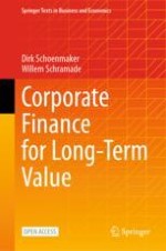
Fundamental valuation methods—through a deeper understanding of companies and their value drivers—are most suited to sustainability integration. This chapter shows how these methods can incorporate social and environmental factors, alongside financial factors, into equity valuation. Moreover, fundamental valuation methods are at the core of valuing S and E in their own right, as discussed in Chap. 5. See Fig. 9.1 for a chapter overview.
4 blocks are labeled sustainable unaware, E S G integrated or inward view, impact or outward view, and integrated value. They have the circles labeled F V, E, and S leading to F V, E V and S V, and F V + E V + S V= I V respectively. They also list a few chapters in each block.
Fig. 9.1
Chapter overview
×
Learning Objectives
After reading this chapter, you should be able to:
Differentiate between absolute and relative equity valuation methods
Perform an equity valuation using various methods
Analyse how fundamental equity valuation brings a deeper understanding of companies and their value drivers
Integrate social and environmental factors into equity valuation
Critically assess alternative valuation methods
9.1 Basics of Equities
Stock markets have captured the imagination of the masses since the spectacular rise and fall of the South Sea Company in the 1720s and perhaps before. Global stock markets reached a market capitalisation of $106 trillion in 2021 (SIFMA, 2021), which is about 125% of global GDP. They perform the important societal function of steering equity finance to productive means. The emergence of the joint stock company has been a great innovation for spreading risk over a large number of shareholders with residual claims and limited liability. Until their emergence, investors could lose more capital than they had put in. The joint stock company lowered financial hurdles (such as liquidity) and helped in steering capital to productive means.
Advertisement
9.1.1 Types of Equity
Stock markets trade public equity, but equity can be private as well. In fact, most equity in most companies starts as private and remains private (see Chap. 10). Only larger companies scale up to become public, because only then the benefits of listing (in terms of risk sharing) start to outweigh the relatively high costs of listing (due to information disclosure requirements). In some ways, private equity investing is instructive for public equity investing. Precisely because private equity lacks standardised data, ratings, and daily pricing, it has not become the victim of benchmark thinking, and reducing companies and portfolios to a few market metrics. Private equity needs to do fundamental analysis of investee companies, which is a good starting point for integrating sustainability into equity valuation.
The way one invests in public equity can be classified as active versus passive investing. Passive investing refers to investments in indices or ETFs (Exchange-Traded Funds, which mimics an index), whereas active approaches tend to be either fundamental (i.e. based on analysis of financial statements, business models, etc.) or quant (i.e. based on factors in a model or algorithm). The attraction of passive investing is that it limits the costs of both trading and analysis. However, it also means there is a very limited scope for the societal allocation role of finance (French, 2008). In fact, as passive investing relies on efficient markets, it is dependent on the presence of sufficient fundamental and quant investors to keep markets efficient. Figure 9.2 provides a classification of public and private equities investing approaches.
A block diagram classifies private and public equity investing approaches. The public approaches include the choice of business fundamentals, the choice of quant factors, and the passive choice of index.
Fig. 9.2
Classification of equities investing
×
Fundamental equity strategiesare rooted in absolute valuation methods from corporate finance and are best suited for sustainability integration. Fundamental investors assess a company, which enables them to identify material sustainability issues and to estimate the impact on the company’s valuation. Fundamental equity strategies are thus the ones with the most potential to integrate sustainability into company valuation. Traditional asset pricing theory has paid limited attention to fundamental equity investing, as it does not align with efficient markets and portfolio theory very well (see Chaps. 12 and 14) and is hard to capture in econometric analysis. That is unfortunate, since fundamental analysis of a company (and its value drivers) is needed to assess the preparedness of companies for the transition to a more sustainable economy. The rise of machine learning can complement fundamental analysis, allowing for the upscaling of fundamental analysis.
9.1.2 Types of Stock Markets
A distinction can be made between primary and secondary stock markets. In the primary market, new issues of a stock are sold to investors. In a secondary market, equities that have been previously issued are traded. When issuing public equity, a firm may obtain a listing on a stock exchange for the first time, the initial public offering (IPO). If a firm is already listed and issues additional shares, this is called seasoned equity offering (SEO) or secondary public offering (SPO).
There are various motives for IPOs. One of the main reasons, of course, is to obtain funds to finance investment. Moreover, the listing of a firm’s shares on a stock exchange increases its financial autonomy, as the firm becomes less dependent on a single financial provider (like a bank). Further, by issuing equity the firm’s owners can diversify their investment risk by selling stakes in the company in a liquid market. Another advantage of public issuance is increased recognition of the company name. In addition, from the moment of the IPO, investors receive better information due to improved transparency and the disclosure requirements that are part of the listing conditions. At the same time, the price of a company’s stock acts as a measure of the company’s value and as a disciplining mechanism for managers.
However, there are a number of inherent disadvantages for a company in listing its shares on a stock exchange. To start with, equity issuance is an expensive procedure, incurring costs such as underwriters’ commission, legal fees, and other charges resulting primarily from the need to satisfy the additional disclosure requirements. From the perspective of investors, going public implies that the ownership of the company is likely to be shared more widely, resulting in a larger gap between external investors and managers. This separation of ownership and control could cause agency problems, where company insiders hold more accurate information on the prospects of the firm than external equity investors, resulting in a divergence of interests between managers and outside investors (see Chap. 3). Lastly, by going public, a company exposes itself to the scrutiny of shareholders, who may be focused too much on short-term results.
9.1.3 Equity Valuation and Its Drivers
There are several methods for determining (or better, estimating) the value of equity. One can distinguish two types of valuation methods:
Absolute valuation methods and
Relative valuation methods
Absolute valuation methods are based on the company’s cash flows. These cash flows are forecasted and then discounted at the company’s discount rate. The dividend-discount model is a basic model that discounts future dividends. An important factor is the expected growth rate of dividends. The discounted cash flow model is more elaborate. It estimates the free cash flows available to equity and bondholders. The equity valuation can be split into three value drivers:
Sales, which can be composed into volumes and price;
Margins, which can be analysed by type of costs and before or after depreciation, taxes, and interest paid; and
Capital, which can be split into the cost of capital (discount rate) and the uses of capital (capex, working capital).
Relative valuation methods derive a company’s value from the value of comparable companies. The idea is to find ‘identical’ companies, which in practice is very difficult, so more or less comparable companies are used. A frequently applied metric is the price-earnings (P/E) ratio, which is the stock prices divided by the earnings. You then multiply your company’s earnings with the P/E ratio of comparable companies. Relative valuation methods are typically used for market transactions (e.g. M&A), as the value is derived from prevailing market prices.
9.1.4 Connecting Equity and Debt Valuation
We can link debt valuation in Chap. 8 and equity valuation in this chapter. To do so, we introduce the concept of enterprise value V0, which is the total value of the company:
The enterprise value is the market value of the company’s underlying business before financing by equity and debt, and separate from any cash. It provides a comprehensive overview of the company’s business activities, which helps to focus on a company’s long-term value, as discussed in Chap. 2. Which activities contribute to the company’s future value and which activities may have a negative impact on the company’s future value? This holistic approach can aid the company in its strategy-setting.
9.2 Valuation Based on Dividends or Free Cash Flows
This section discusses two absolute equity valuation methods: the dividend-discount model and the discounted cash flow model. The second method is at the heart of fundamental equity valuation.
9.2.1 The Dividend-Discount Model
The dividend-discount model looks at cash flows to equity investors. A first cash flow is the dividend that an investor receives. A second cash flow is the cash received when selling the stock at some future date. Taking the perspective of a 1-year investor, we get the following equation for today stock price P0:
Today, stock price P0 is the net present value of the dividends received during the year Div1 and the stock price at the end of the year P1. These cash flows are discounted at the cost of equity rE, which is the expected return of other investments available in the market with similar risks. We can rewrite Eq. (9.2) as follows:
The total return of the stock for the equity investor can thus be split in the stock’s dividend yield and the stock’s capital gain. Example 9.1 shows how the stock price and return of a company can be calculated.
Example 9.1: Calculating Stock Price and Return
Problem
We assume that Unilever, a global consumer goods company, will pay dividends of €1.40 per share and trade at €46 per share at the end of the year. If the cost of equity is 7%, what would you be prepared to pay for Unilever today? What dividend yield and capital gain are expected?
Solution
Using Eq. (9.2), we can calculate today’s stock price:
So, today’s stock price would be €44.30. The dividend yield is \( \frac{Div_1}{P_0}=\frac{1.40}{44.30}=3.2\% \) and the capital gain is \( \frac{P_1-{P}_0}{P_0}=\frac{46.00-44.30}{44.30}=3.8\% \). The dividend yield and the capital gain add up to the total return: 3.2% + 3.8% = 7.0%, which is equal to the cost of equity.
Up till now we use 1 year’s dividend and the stock price at the end of the year (at which you can sell the stock in the market) to calculate today’s stock price. Instead of referring to future stock prices, we can expand the dividend-discount model to a multiyear perspective:
So, the stock price is equal to the present value of the expected dividends. As the company develops, its earnings and dividends are expected to grow. Assuming a constant dividend growth g, we get the following:
We can now use Eq. (4.6) from Chap. 4 for valuing a perpetuity. This is the present value of a continuous stream of constant cash flows: \( PV=\frac{CF}{r} \). In this case, we have growing dividends (instead of constant dividends). The equation is then as follows:
$$ {P}_0=\frac{Div_1}{r_E-g} $$
(9.6)
This is the famous constant dividend growth model. Dividends cannot keep on growing beyond the discount rate forever, as this would imply an infinite stock price (i.e. value) of the company. So, this formula requires that the constant growth rate of dividend is below the discount rate. Example 9.2 shows how we can value a company with constant dividend growth.
Example 9.2: Valuing a Company with Constant Dividend Growth
Problem
E.ON is a European electric utility provider based in Essen, Germany. E.ON pays 40 euro cents (€.40) in dividend. The cost of equity is 6% and dividends are expected to grow with 2%. What is E.ON’s stock price?
Solution
Using Eq. (9.6), we can calculate today’s stock price:
The earnings per share EPS is the company’s earnings divided by the number of outstanding shares. The dividend is thus the EPS multiplied by the payout ratio, which is defined as payouts divided by earnings or net income (see Chap. 16). Equation (9.7) shows that dividends are ultimately based on a company’s earnings. So, there is natural limit to dividend growth, as the underlying earnings matter. Next, there are dangers in constant growth formulas. As circumstances change, the growth of dividends (and underlying earnings) will change. High-growth companies, for example, are not likely to keep these growth rates forever. This is the fallacy of extrapolating current numbers, without thinking about whether these numbers can be sustained in the future.
An update of the original dividend growth model includes share repurchases. Companies complement dividend payouts with share repurchases, because share repurchases are exempt from dividend tax. Share repurchases are therefore a more tax-efficient way of rewarding shareholders. The economic effect is the same. This is because shareholders are still entitled to future earnings, which are now assigned to the remaining shares (the originally outstanding shares minus the repurchased shares), so that each shareholder’s claim on future earnings remains the same. The total payout model includes both dividends and share repurchases:
So, the equity value is the present value of total dividends and share repurchases.
9.2.2 The Discounted Cash Flow Model
Another absolute valuation method is the Discounted Cash Flow (DCF) model. It goes several steps further than the Dividend-Discount Model, which only estimates the resulting cash flows from the business operations paid as dividends to shareholders. The Dividend-Discount model thus measures the company’s equity value. The DCF model values a company’s assets on the basis of their discounted future cash flows. It covers the enterprise value, which is the sum of a company’s equity and debt (see Eq. 9.1).
To value the enterprise, we start with estimating the free cash flows that the company has available for all investors: equity and debt holders. Company cash flows can be estimated in the same way as project cash flows in Chap. 7. The starting point is the earnings before interest and taxes EBIT. The company has to pay corporate tax τ on these earnings. These items are based on accounting. The next step to arrive at cash flows is to deduct net investment and increases in net working capital NWC (see Chap. 7 for a definition of NWC). Net investment and increases in NWC support the company’s future operations and growth. A company’s net investment is defined as the company’s capital expenditures CAPEX minus depreciation:
FCF is the cash flow left to be distributed to financiers after all positive NPV investments have been done. It is calculated as cash from operations minus cash into investments. It is important to use FCF rather than earnings which is much more easily manipulated, as is visible in accruals. Accruals are differences between net earnings and operational cash flow, driven, for example, by revenues or expenses that have been earned or incurred (in other words ‘accrued’ to the accounts), but cash related to the transactions has not yet changed hands. Another factor which can be manipulated is depreciation. A company can increase depreciation to reduce (taxable) profits or decrease depreciation to show higher book profits to investors. In that way, companies can smooth profits over time, which is also referred to as ‘cooking the books’. Cash flow statements can overcome these accounting gimmicks. Deprecation is, for example, deducted as a cost item in EBIT, but subsequently added to CAPEX to derive net investment. Depreciation is thus eliminated from the cash flow analysis.
The free cash flow FCF can be discounted to obtain the enterprise or company value V0 at t = 0:
where WACC represents the weighted average cost of capital and TVN the terminal value at t = N, which may in turn be valued with a DCF (see below Eq. 9.14). Note that V0 in the DCF formula is the enterprise value of the company to all financiers, i.e. the value of debt and equity together. Equity holders are residual claimholders, who receive income only after the debt holders have been paid. In effect, equity is a call option on the company (Merton, 1974; see Chap. 19 on options).
WACC is the weighted average cost of capital, which is the rate of return demanded by the company’s financiers (of both equity and debt) and is derived from the expected return on an asset with similar risk (see Chap. 13 on WACC).
In the case of a constant growth g of the company’s FCF from t = 0, we can simplify Eq. (9.12). Just like in the dividend-discount model (Eq. 9.6), the value V0 of the constant stream of growing free cash flows can be summarised as follows:
$$ {V}_0=\frac{FCF_1}{WACC-g} $$
(9.13)
In a similar way, we can calculate the terminal value TVN in Eq. (9.12) as follows:
$$ T{V}_N=\frac{FCF_{N+1}}{WACC-g} $$
(9.14)
A constant growth rate of the company’s cash flows FCF is a simplifying assumption. A DCF valuation crucially relies on assumptions to be made on future FCF and on the cost of capital WACC, as well as on their elements. This opens the door to a behavioural problem, because analysts often simply extrapolate recent historical numbers or short-term forecasts into infinity (while the company is exposed to internal and external changes which impact it).
The DCF example in Table 9.1 illustrates how that works. The top part lists the inputs (e.g. a sales growth of 6 per cent until 2030, a long-term sales growth of 2%, and an EBIT margin of 11–12%) and the components (sales, EBIT, and taxes) to calculate the FCF. The note at Table 9.1 explains the abbreviations. First, taxes are deducted from EBIT to obtain the net operation profit less adjusted taxes (NOPLAT). Next, depreciation is added (no cash outflow) and investment in the form of CAPEX and NWC is deducted (cash outflow) to obtain the FCF. The rows represent the years: the shaded area from 2023 to 2031 are the assumptions made by the analyst to arrive at the forecasted cash flows (all other data in Table 9.1 is given or calculated). The middle part contains the discount factor (based on a WACC of 8%) to discount the FCF to the present value.
Table 9.1
DCF valuation with the value drivers—analyst extrapolation
A table of values lists the sales growth, E B T margin, tax rate, depreciation per sales, C A P E X per sales, N W C per sales, sales, E B T, taxes on E B T, N O P L A T, and more, for W A C C for F Y 2019 to F Y 2022 and for T V from F Y 2023 e to 2031 e.
Notes: FY2019–FY2022 relate to the historical financial performance of the company. 2023e–2031e are projections of future financial performance, made by the analyst. WACC is the weighted average cost of capital, the rate at which the company’s cash flows are discounted. TV growth is the assumed growth rate after the explicit forecast period, where TV is the terminal or continuing value. EBIT is earnings before interest and taxes, also known as operating profit. CAPEX is the capital expenditure made by the company. NWC is net working capital, i.e. short-term liquid assets minus short-term finance. NOPLAT is net operating profit less adjusted taxes. Gross CF is the cash flow before investment. FCF is the free cash flow to the company. ROIC is return on invested capital
The enterprise value V0 is the sum of the present values of the free cash flows from 2023 to 2030 and the terminal value. Next, net debt is deducted and cash added to obtain the equity value (Eq. 9.1). Dividing the equity value by the number of shares outstanding provides the stock price:
Finally, the bottom part outlines the capital side: net working capital NWC, invested capital, and return on invested capital (ROIC). The invested capital is net investment (from Eq. 9.10) and NWC. The return on invested capital is the net operation profit less taxes divided by invested capital:
Some argue that short-termism is not an issue, as stocks incorporate more than a decade of cash flows in their pricing. That is true, but cash flow forecasts can be a mere extrapolation of the short term—not reflecting change or the relevance of sustainability. Multiples (relative) valuation in Sect. 9.3 faces this problem as well, and to an even larger extent, as it implicitly makes the same assumptions while giving the analyst a false sense of being objective.
In a DCF valuation, one can make explicit assumptions and choose to be very clear on which point one disagrees with the market. In a DCF valuation of the same company as in Table 9.1, an analyst uses, for example, exactly the same assumptions with one crucial difference: since they have a stronger belief in the company’s competitive position, their margin assumptions are 4% higher (an EBIT margin of 16 instead of 12%), resulting in a 35% higher fair value of the stock.
The full DCF valuation model in Table 9.1 is the bread and butter of a seasoned equity analyst, but it is also quite elaborate. To provide more practice and the ability to develop a more intuitive understanding, we give a simpler valuation example. Example 9.3 calculates the value of Adidas’ stock price at €301.2. Since the calculation of the value depends on several assumptions on sales, EBIT margins, investment needs, and cost of capital, Example 9.4 provides a sensitivity analysis of Adidas’ stock valuation. The sensitivity analysis shows that ‘under reasonable assumptions’ the stock price can fluctuate from –24% (€227.6) to +28% (€385.5) in comparison with the midpoint estimate of €301.2.
Example 9.3: Valuing Adidas Using Free Cash Flow
Problem
Adidas, a German sportswear manufacturer, has sales of €19,844 million in 2020. We make the following assumptions. First, a sales growth of 9% until 2025 and a long-term sales growth of 3% (industry average). Next, the EBIT margin is expected to be 13% based on past margins and the effective tax rate is assumed to remain 26% in Germany. Finally, net investments and increases in NWC are, respectively, expected to be 4 and 8% of any increases in sales based on past investment needs. Adidas has €3597 million in excess cash, €2295 million in debt and 195 million shares outstanding. If the WACC is 7%, what is your estimate of the value of Adidas’ stock price in early 2021?
Solution
Using Eq. (9.11), we can calculate Adidas’ free cash flows based on the assumptions (in italics) as follows:
Year
2020
2021
2022
2023
2024
2025
Free cash flow forecast (€ millions)
Sales
19,844.0
21,630.0
23,576.7
25,698.6
28,011.4
30,532.5
Growth versus previous year
9%
9%
9%
9%
9%
EBIT (13% of sales)
2811.9
3065.0
3340.8
3641.5
3969.2
Less: Income tax (26% EBIT)
–731.1
–796.9
–868.6
–946.8
–1032.0
NOPLAT
2080.8
2268.1
2472.2
2694.7
2937.2
Less: Net investment (4% ofincrease in sales)
71.4
77.9
84.9
92.5
100.8
Less: Increase in NWC (8% ofincrease in sales)
142.9
155.7
169.8
185.0
201.7
Free cash flow
1866.5
2034.5
2217.6
2417.2
2634.7
As we expect Adidas’ free cash flow to grow at a constant rate of 3% after 2025, we use Eq. (9.14):
Example 9.4: Sensitivity Analysis for Adidas’ Stock Valuation
Problem
In Example 9.3, Adidas’s sales growth rate was assumed to be 9% and the EBIT margin 13%. The valuation very much depends on these assumptions. What would Adidas’ stock price be with sales growth of 8% until 2025? And what would the stock price be if, in addition, the EBIT margin is 12%?
Solution
The basis answer is that we can redo the calculation of Adidas’ stock price with the new assumptions. The set-up of the calculation remains the same as in Example 9.3, only the inputs change. Luckily, that can quite easily be done in an Excel spreadsheet by changing the parameters for sales growth and EBIT margins.
Depending on the inputs, the stock valuation is as follows:
Sales growth
7%
8%
9%
10%
11%
11%
227.6
238.9
250.7
262.8
275.4
12%
250.7
263.1
275.9
289.2
302.9
EBIT
13%
273.9
278.3
301.2
315.5
330.4
Margin
14%
297.1
311.5
326.4
341.9
357.9
15%
320.2
335.7
351.7
368.3
385.5
At the time of analysis (Autumn 2021), Adidas’ stock price was valued close to €301.2 based on 9% sales growth and 13% EBIT margin. A decrease of sales growth to 8% would give a stock price of €278.3. A reduction in EBIT margin to 12% in addition would yield a stock price of €263.1. This is a reduction in stock price of 13% compared to the previous assumptions of 9% sales growth and 13% EBIT margin. The table confirms that the stock valuation is very sensitive to the inputs—ranging from €227.6 (–24% based on 7% sales growth and 11% EBIT margin) to €385.5 (+28% based on 11% sales growth and 15% EBIT margin).
9.2.3 Comparing Absolute Valuation Methods
We can compare the different absolute stock valuation methods. Table 9.2 summarises the various discounting methods with increasing information needs. The dividend-discount model estimates the dividend payments per share to derive a company’s stock price. As share repurchases are becoming more important, the total payout model includes total dividends and share repurchases to calculate a company’s equity value. These are relatively easy to establish.
The most cumbersome, but insightful method is applying the full discounted cash flow model to establish a company’s enterprise value. One needs to estimate a company’s free cash flows and then its weighted average cost of capital. As Table 9.1 shows, this is quite an exercise. The benefit is a fundamental valuation of the company. The discounted cash flow model is also the basis for calculating a company’s integrated value in Sect. 9.5.
9.3 Valuation Based on Comparable Companies
Absolute or fundamental valuation methods are based on discounting a company’s cash flows. By contrast, relative valuation methods derive a company’s value from comparable companies, often in the same industry.
9.3.1 Equity Value Multiples
In the case of relative valuation, often called multiples valuation, a stock value P0 (or more generally, an asset’s value) is derived from the given (market) value of another comparable stock. For example, a fast moving consumer goods company like Unilever might be valued by taking its earnings per share EPS0 and multiplying that number with the average price-earnings P/E ratio of its peer group:
$$ {P}_0={EPS}_0\ast \frac{P}{E} $$
(9.17)
So, in this method, when Unilever’s EPS is €2.2 and its peers trade at a P/E of 24.0 at year-end 2021, then Unilever’s fair stock value P is 24.0 × €2.2 = €52.8. Table 9.3 shows the average P/E of Unilever’s direct peers from the consumer goods industry. Unilever’s stock price is €46.8 at year-end 2021. So, Unilever’s P/E ratio is slightly lower at 21.3 than the industry average at 24.0. Example 9.5 shows how Apple’s stock price can be derived using the technology’s industry’s P/E ratio.
Table 9.3
Stock price, price-earnings (P/E), and market price-book (P/B) at year-end 2021
Company
Stock price
P/E
P/B
Comparable companies
P/E
P/B
Unilever
€46.8
21.3
6.8
Danone
16.9
2.1
Kraft Heinz
20.0
0.9
Procter & Gamble
29.7
8.7
Nestlé
29.2
7.5
Average
24.0
4.8
The P/E ratio can be used to derive a company’s equity value by multiplying the stock value from Eq. (9.17) with the number of outstanding shares. The P/E ratio is thus an equity value multiple.
Forward P/E Ratio
A disadvantage of using the P/E ratio is that a company’s current earnings can be distorted, because of exceptional circumstances related to the company (e.g. a reorganisation) or the economy (e.g. the covid-19 pandemic). A way to address that is by using forward earnings, which are the expected earnings over the next 12 months. Forward P/E ratios are more suitable for valuation purposes.
Price to Book Ratio
Another method using the stock price is the market price to book value ratio P/B. This ratio divides the market value by the book value of equity. Table 9.3 indicates that the P/B ratio of the consumers goods industry fluctuates from 0.9 for Kraft Heinz to 8.7 for Procter & Gamble. This wide fluctuation makes the price-book ratio very imprecise and thus less reliable for comparing company values. In practice, the price-earnings ratio is the most commonly used method for multiples valuation.
The problem with relative valuation is that it relies on fair valuation of the comparable assets, which in practice are not necessarily priced correctly. Another disadvantage is that it can be quite hard to find companies that are comparable, meaning that there are no perfect substitutes for a company. Each of its competitors is, for instance, active in different geographies, different segments and serves different customers, which may impact the P/E ratio. Moreover, companies may have different growth rates and EBIT margins.
Another problem is that industries can be overvalued. An example is the boom in Internet stocks in the late 1990s and early 2000s, before the Internet bubble burst. While multiples could justify the value of these companies in relation to each other, it was more difficult to justify the stock prices of these companies jointly (Berk & DeMarzo, 2020).
Example 9.5: Valuation Using the P/E Ratio
Problem
Suppose big tech company Apple has earnings per share of $5.8 at year-end 2021. The technology industry’s price-earnings ratio is 27.7. What is Apple’s stock price using multiples valuation? How does that compare to Apple’s current stock price of $177.6 at year-end 2021?
Solution
Using Eq. (9.17) provides Apple’s estimated stock price:
So, the multiples valuation of $160.8 gives a lower stock price than the actual stock price of $177.6. Apple’s P/E ratio is higher than the industry’s average. This highlights that multiples valuation is an approximation.
9.3.2 Enterprise Value Multiples
Companies differ also in leverage, making more leveraged companies riskier. That makes a precise comparison between companies difficult. To correct for leverage, multiples can be based on a company’s enterprise value V. As enterprise value is the company’s value before financing, the earnings should also be adapted to an earnings number before payment to financiers. A common earnings indicator is earnings before interest and taxes EBIT. In case one wants to correct for investments as well, earnings before interest, taxes, depreciation, and amortisation EBITDA can be used. The multiples formula for enterprise value V0 is as follows:
$$ {V}_0=E{BITDA}_0\ast \frac{V}{EBITDA} $$
(9.18)
Whereby V/EBITDA is the enterprise value multiple.
To get a company’s stock price P0, we need to deduct net debt from enterprise value to get a company’s equity value and subsequently divide that by the number of shares outstanding (see Eq. 9.15).
9.4 Impact of S and E on F: Integrating Sustainability into Value Drivers
A high-level and pragmatic way to integrate sustainability into enterprise valuation is to adjust the value drivers on material sustainability issues. This gives a first-order approximation of the financial value (FV) consequences of sustainability. The value driver adjustment approach provides the inward perspective on sustainability and is financially driven (see Fig. 9.3, which is a reproduction of Fig. 2.6 from Chap. 2).
A cyclic illustration of inward dependencies and outward impacts between society and nature and business and financial values.
Fig. 9.3
The inward and outward perspective on company valuation
×
Section 9.5 takes the outward perspective on sustainability, estimating a company’s social and environmental impact (SV and EV). Estimating the social and environmental value components is more elaborate and data-intensive. The calculation of the value components allows us to establish the company’s integrated value in Sect. 9.5, which is a combination of financial value (FV), social value (SV), and environmental value (EV).
9.4.1 Value Driver Adjustment Approach
While academic corporate finance is very much concerned with risk and discount rates (see Chaps. 4 and 12), it tends to take a company’s free cash flow as a given and it does not analyse where that free cash flow comes from. Fundamental equity valuation methods, like the DCF model in Sect. 9.2, analyse both cash flows and discount rates. Schramade (2016) introduces the Value Driver Adjustment (VDA) approach to integrate sustainability into the DCF model. The starting point is to split the enterprise valuation into value drivers (Koller et al., 2020):
Sales, which can be composed into volumes and price
Margins, which can be analysed by type of costs and before or after depreciation, taxes, and interest paid, and
Capital, which can be split into the cost of capital (discount rate) and the uses of capital (capex, working capital)
While the first two value drivers (sales and margins) affect cash flows, only the third value driver (capital) affects the discount rate. Making these splits in value drivers can yield useful insights into how efficiently and successfully a company is run. Moreover, one can also analyse what is driving the value drivers. That is, what are the sources of competitive advantage that determine how fast a company grows and how profitable it can sell its goods and services (see Chap. 2). This is also where the link to sustainability comes in, as intangible assets on material social and environmental issues (such as intellectual capital, social capital, or environmental capital) tend to be the underlying value drivers.
Think of a mining company that has much lower costs than its peers because it is much better at managing local stakeholders (and hence experiences less delays and production losses) and has a better safety record (and more efficient production). Then consider a mining company that currently enjoys lower costs than its peers because it is ignoring lots of safety regulations and is paying its employees poorly, without pension or social security arrangements. That cost advantage is likely to be temporary and entails a high risk of costly disruptions, which should be factored into its cost of capital.
Applying the VDA approach, Schramade (2016) proposes a three-step approach to integrating sustainability into fundamental enterprise valuation:
1.
Identify and focus on the most material issues
2.
Analyse the impact of these material factors on the individual company
3.
Quantify competitive advantages to adjust for value driver assumptions
Step 1: Identify and Focus on the Most Material Issues
Since material social and environmental factors, by definition, can have a substantial impact on business models and value drivers, analysts should take them into account in their valuation models. One needs a disciplined approach to identify material sustainability factors in the first place (see Chap. 5). Ideally, one does a materiality analysis of the industry (or has such analyses at one’s disposal for all industries), plotting the likelihood of impact of a social or environmental issue against its likely size.
For a mining company for example, one could identify management of local stakeholders, environmental management, and operational health and safety as material issues. For a pharmaceutical company, the likely material issues are innovation management, human capital management, and product quality and safety. Then for a particular mining or pharmaceutical company, the importance of an issue can be more or less important than for the industry overall. For example, operational health and safety tends to be even more important for more manual types of mining (such as gold or platinum) than for more mechanised types of mining such as are typically found in iron ore mining.
Step 2: Analyse the Impact of These Material Factors on the Individual Company
After establishing the material social and environmental factors, the analyst draws up an assessment of the company’s performance on these factors. Such analysis is not only done on an absolute basis, but also relative to peers, which is critical when establishing whether a company enjoys a competitive advantage (or disadvantage) in managing a given sustainability issue. For example, Novozymes’ competitive edge in human capital and innovation management means that it is able to attract the best talent in enzymes (see Box 9.1). At the other side of the spectrum, Anglo American’s weak management of local stakeholder relations results in serious local opposition to projects, operational mistakes, and long delays in project ramp-ups (see Box 9.2).
Step 3: Quantify Competitive Advantages to Adjust for Value Driver Assumptions
In the next step, the equity analyst makes deliberate, and often significant, adjustments to value drivers that are based on the sustainability-driven competitive advantages or disadvantages. These changes in value driver assumptions result in changes to the target price of the company’s stock. To give a sense of magnitudes, if the analyst raises profit margins for all periods from 20 to 23% (that is, a 15% increase) to reflect the company’s proficiency in managing a sustainability issue, the target stock price will likely also go up by 15%. In the case of Novozymes, the impact was much bigger, as its competitive edge in innovation and talent result in superior products that replace traditional chemicals—at double the margins and double the growth rate of the traditional chemicals industry (see Box 9.1).
Box 9.1: Novozymes: Competitive Advantage from Innovation
Novozymes is a Danish enzyme maker that replaces traditional chemicals with enzymes (proteins that act as catalysts) in, for example, washing powders, baking and agricultural products. Its enzymes provide better performance at lower temperatures and hence lower energy costs and lower emissions. As a result, the company is growing twice as fast and at double the profit margin compared to ordinary chemicals companies. Novozymes’s growth and margins are driven by innovation, which depends in turn on human capital. Figure 9.4 illustrates the value drivers of Novozymes.
A block diagram. The valuation includes sales growth, margins, and capital. Sales growth and margins lead to innovation, which leads to human capital.
Fig. 9.4
Value drivers of Novozymes. Note: The scheme shows the value drivers in a bottom-up way
×
Box 9.2: Anglo American’s Failure to Manage Local Stakeholders
Mining companies use a lot of capital to build and maintain mines that tend to be in operation for decades. All of that is wasted if the company loses its licence to operate due to environmental problems or unresolved local stakeholder conflict. Figure 9.5 shows the value drivers of a mining company.
A flow diagram of valuation. Valuation points to sales growth, margins, and capital. Sales growth leads to price and production volume. Production volume, margins, and capital point to the management of local stakeholders and environmental management.
Fig. 9.5
Value drivers of a mining company. Note: The scheme shows the value drivers in a bottom-up way
×
South African mining company Anglo American has a long history of technical expertise and strong project execution. However, because the associated intangible human resources were neglected, many people left the firm, and much of its corporate memory was lost. The result was weak execution on projects. The Minas Rio iron ore project in Brazil turned out to be especially disastrous: originally planned to be built for around $2.5 billion, the project was delivered years over deadline and about $10 billion over budget. Local conditions were not sufficiently analysed and necessary environmental permits were not applied for. While Anglo had high scores with sustainability ratings agencies, and scored well on many immaterial issues, it failed spectacularly on its most material sustainability issues: local stakeholder management and environmental management.
The VDA approach is very practical. Box 9.3 provides a case study of a medtech company (based on a list of questions summarised in the Appendix to this chapter). The combined insights from sustainability analysis and traditional fundamental analysis allow one to make better financial valuations. Schramade (2017) argues that the impact can be substantial and reports valuation impacts ranging from –23% to +71% for a sample of 127 investment cases. Value driver adjustments can be made on any sustainability issue, but some are more frequent than others. Innovation, corporate governance, environmental management, and supply chain management are frequently used. The way value driver adjustments are made also differs: while value driver adjustments on innovation tend to be made to sales growth and margins (reflecting competitive position), the value driver adjustments on corporate governance are mostly about adjusting the cost of capital (reflecting risk).
Box 9.3: VDA Example
For a medical technology company, the three steps of the VDA approach are as follows (see the Appendix for the underlying questions):
1.
Identification of material issues For the industry, the analyst identified the following issues as material: innovation management; human capital management; and energy efficiency & circular economy.
2.
Performance on material issues The analyst assessed the medtech’s key strengths to be in innovation management, human capital and capital management, while the others are too close to call.
3.
Make value driver adjustments The analyst estimated that the medtech’s strong focus on digital innovation puts the company ahead of the competition and could boost sales growth by 1% and that the medtech’s innovation and circularity/energy savings could help drive the company’s margins by as much as 2%. The net result of these effects is an increase in target price of 22% from 39.3 to €48.1.
Innovation and circularity/energy savings: +200 bps
No impact: 0 bps
€8.8 (22% higher value)
Total
5%
15%
8%
€48.1
The above illustrations of the VDA approach do not include a transition perspective. But the transition perspective can be included by building transition scenarios with distinctive value driver assumptions. Please see the Inditex case study in Chap. 11 (Sect. 11.3) for an illustration of how that works.
9.5 Valuation of S & E and Integrated Value
As stated in Chap. 8, the valuation of S and E is similar to the valuation of F at enterprise level. In this set-up, FV is enterprise value, which is the sum of equity and debt. S and E are valued separately and are a result of the company’s operations. Integrated value is simply the sum of FV, EV, and SV—see Fig. 9.6.
A block diagram of integrated value. The components of integrated value are F V enterprise value, E V, and S V. The F V includes equity and debt. E V is the value of E times the price. S V is the value of S times the price.
Fig. 9.6
The components of integrated value
×
For both SV and EV, the value calculation can be done in the three steps presented in Chap. 5:
1.
Determine material S and E issues
2.
Quantify the S and E issues in their own units Q and
3.
Put a monetary value on those S and E units with shadow prices SP
See Chap. 5 for an elaboration of these three steps. The valuation is done in the DCF way as described in Sect. 9.2.3.
Figure 9.7 shows what the composition of integrated value, and in it the role of equity (assets minus debt), might look like for a company. In this hypothetical case, equity looks fine (35), because of limited leverage: debt (25) is not very high compared to assets (60). But the company looks vulnerable due to large negative values for S and especially E, which raise the risk of the company and its equity. These effects of leverage from E and S will be discussed further in Chap. 15 on capital structure.
A positive-negative bar graph of the value of equity shares versus components of a company's integrated value. The labels and their values are as follows. E V +, 2. E V minus, minus 30. S V +, 8. S V minus, minus 14. Debt, 25. Equity 35. Values are estimated.
Fig. 9.7
The components of integrated value & share of equity for company X
×
In addition, you should be aware that these types of value can spill over into each other. The social and environmental value can be internalised (i.e. spillover) in the financial value, as shown in Chaps. 6 and 7. Chapter 11 provides an in-depth case study to show how the integrated value of a company can be calculated.
9.6 Conclusions
A company’s enterprise value refers to the value of its business activities, which are financed by equity and debt. Chapter 8 already covered the methods to value and price bonds (debt). This chapter examines methods to derive the value of public equity (these are listed stocks; see Chap. 10 for private equity). These equity valuation methods either look at a company’s ‘fundamentals’ or compare a company to a similar company, in order to obtain a company’s value.
In the first case, absolute valuation models are fundamental methods to calculate value by discounting cash flows from business activities or discounting dividends which are paid from realised profits. The discounted cash flow model is well placed to integrate sustainability into valuation. By contrast, relative valuation models determine the value of one company in comparison with another company with similar characteristics. With a few market metrics, a company’s value can then be derived.
Sustainability matters more to equity valuation than most equity investors realise. Material sustainability issues can make or break companies. As residual claimholders, equity investors bear most of the risk when companies fail and they also reap most benefits when companies succeed. Therefore, equity investors have strong incentives to help companies achieve the conditions for integrated value creation described in Chap. 2.
Fundamental valuation methods—through a deeper understanding of a company’s value drivers—are most suited to sustainability integration. This chapter shows how these methods can incorporate social and environmental factors, alongside financial factors, into equity valuation.
Key Concepts Used in This Chapter
Absolute valuation is a valuation of an asset without reference to the valuation of other assets; absolute valuation methods are based on a company’s cash flows
Accruals are adjustments for revenues earned and expenses incurred that are not yet recorded in the accounts
Discounted Cash Flow (DCF), also known as Net Present Value (NPV), is a method that values an asset or project by calculating cash flows and discounting them at a risk-adjusted discount rate
Enterprise value is the market value of the company’s underlying business before financing by equity and debt and separate from any cash
ESG refers to environmental, social, and governance
ESG integration is the explicit integration of E, S, and G issues into the valuation and selection of securities
Exchange-Traded Funds (ETFs) are vehicles for passive investing
Fair value is an assessment of the value of an asset according to a (relative or absolute) valuation method, which may deviate from the asset’s current price
Fundamental analysis is an approach to investing based on obtaining a good understanding of a company’s business model and valuation
Materiality is the relevance of a certain issue to value creation
Multiples valuation is a type of relative valuation in which an asset’s value is determined as a multiple of a financial statement metric such as profitability or book value
Net Present Value (NPV), also known as Discounted Cash Flow (DCF), is a method that values an asset or project by calculating cash flows and discounting them at a risk-adjusted discount rate
Passive investing is an approach to investing that buys widely diversified portfolios, often made up of entire market indices, and limits the amount of buying and selling, so as to steadily build wealth over time
Payout ratio is payouts (in the form of dividends and/or share buybacks) divided by earnings or net income
Private equity is the equity of privately held companies
Public equity is the equity of companies listed at a stock exchange, also called publicly listed companies
Quant investing is an investment approach that selects securities using advanced quantitative analysis
Relative valuation is a valuation of an asset with reference to the valuation of other assets; relative valuation methods derive a company’s value from the value of comparable companies
Valuation is the process of arriving at a value estimate
Value drivers are the main components of valuation and its formula, namely sales growth, profit margins, cost of capital, and investment
Value Driver Adjustments (VDA) are the adjustments made to value driver assumptions in a valuation model, based on an assessment of the company’s material ESG issues
Weighted Average Cost of Capital (WACC) is the minimum required return on a company’s investments given its risk profile
Open Access This chapter is licensed under the terms of the Creative Commons Attribution 4.0 International License (http://creativecommons.org/licenses/by/4.0/), which permits use, sharing, adaptation, distribution and reproduction in any medium or format, as long as you give appropriate credit to the original author(s) and the source, provide a link to the Creative Commons license and indicate if changes were made.
The images or other third party material in this chapter are included in the chapter's Creative Commons license, unless indicated otherwise in a credit line to the material. If material is not included in the chapter's Creative Commons license and your intended use is not permitted by statutory regulation or exceeds the permitted use, you will need to obtain permission directly from the copyright holder.
Appendix: Case Study Template—How to Integrate Sustainability into Financial Valuation
This case study template allows you to do your own sustainability integration analysis for estimating a company’s enterprise value using the Value Driver Adjustment (VDA) approach of Sect. 9.4. The list of questions in this case study has been made over the course of several years of doing sustainability integrated investment analysis. The questions have been structured as an assignment for the Sustainable Finance course taught at Rotterdam School of Management, Erasmus University, and can be found in Principles of Sustainable Finance (Schoenmaker and Schramade, Oxford University Press, 2019, Chapter 8).
The questions will deepen students’ and practitioners’ understanding of sustainability integration by having them apply sustainable finance insights to a real-life example—and ideally discuss with fellow students, teachers, or colleagues. The list contains a set of questions in six sections. Although the six sections address different issues, it should become evident during the analysis that they are related. To answer the questions, students have to rely on a company’s reports (among other documents). Please make sure you read these documents with a critical mind; do not take all the company’s messages at face value and look for independent sources. For the valuation questions, please include your Discounted Cash Flow calculation (see Sect. 9.2).
A.1 Business Model and Competitive Position
See Chap. 2 for a description of the business model and competitive position.
How would you describe the company’s business model?
How strong do you rate the company’s competitive position?
What trends affect the company’s business model and competitive position?
A.2 Value Drivers: Part 1
See Sect. 9.4 for the value drivers—sales growth, margins, and capital.
On sales growth:
What seems to be a typical sales growth for the company? Please explain. Furthermore, what are the drivers of sales growth?
On margins:
What seems to be a profit margin (EBIT or EBITDA) for the company? Please explain. In addition, what are the drivers of that margin?
On capital:
How capital intense is the company? Please explain
What do you think is the firm’s cost of capital? Please explain
Valuation of company (based on enterprise value):
What is the fair value (based on your DCF calculation) of the company?
Value driver
Assessment for next decade
Sales growth
Margins
Capital (WACC)
DCF value
A.3 Sustainability
See Chaps. 2 and 5 for the key sustainability concepts.
Purpose:
What is the company’s purpose/reason for being? In what way does the company create value for society? How does it get paid for that value creation?
Stakeholders:
What are the company’s main stakeholders? Please fill out the stakeholder impact tool below:
Material issue
Stakeholder 1
Stakeholder 2
Stakeholder n
Short-term goals
Long-term goals
How the company helps those goals
How the company hurts those goals
Externalities and impact:
Does the company generate serious externalities? Are they positive or negative? How do you assess the chances of these externalities to be internalised?
Which of the SDGs (if any) does the company help achieve? Which negative SDG exposures (if any) does the company have?
To what extent can the company’s impact be measured? Does the company report on its impact? How can its reporting be improved?
Material issues:
What are the most material sustainability (S and E) factors? I.e. what issues are most critical to the success of the company’s business model? Please fill out the below matrix, discussing for each of these most material S and E factors (1) how the company performs on it; (2) whether the company derives a competitive (dis)advantage from it; (3) how they might affect the value drivers
Material issue
Performance
Competitive edge?
Impact on value drivers?
Issue 1
Issue 2
Issue 3
Issue 4
A.4 Strategy and Reporting
See Chap. 2 for company strategy and Chap. 17 for sustainability reporting.
How would you describe the strategy of the company?
To what extent does that strategy take into account the company’s most material sustainability issues? Please link to your answer in Sect. A.3.
Is the strategy consistent with the company’s purpose? Please explain.
How do you assess the company’s sustainability reporting?
A.5 Value Drivers: Part 2
Section 9.4 shows how the below VDA tables can be filled in for a company (e.g. Box 9.3).
Given all of the above questions and your answers, how do you rate the effect of material sustainability issues on the value drivers going forward?
For each value driver, please indicate whether you see a positive, negative, or neutral effect—and please explain why.
Value driver
Positive/negative/neutral
Explanation
Sales growth
Margins
Capital (WACC)
How would this affect your valuation of the company? Please provide the details of your DCF calculation excluding and including sustainability (S and E) (dis)advantages.
Value driver
Company excl. S and E (dis)advantages (in %)
Company incl. S and E (dis)advantages (in %)
Company (dis)advantage (in basis points)
Sales growth
Margins
Capital (WACC)
DCF value
A.6 Investment Conclusions
In sum, how attractive do you find the company as an investment? Please explain and refer to your answers above.
How would you compare the sum of your facts/findings with the overall impression you get of the company’s transition preparedness?
Suppose you were in the role of advisor to this company. Which strategies might the firm take to improve its transition preparedness? Which obstacles would you foresee in taking those steps?
Would you say the company is part of the problem or part of the solution in the transition to a sustainable economy? Substantiate your answer.