Financial options are contracts that give the owner the right to buy (in the case of a call option) or sell (in the case of a put option) a security at a pre-specified price (the exercise price). The flexibility is on the side of the buyer, but the seller is compensated with a premium paid by the buyer. Sophisticated models have been developed to determine the value of options. Options are interesting since they offer an alternative way of tying payoffs to (future) situations, also outside of contractual settings. In that case, they are called real options. Real options come in various types, such as the option to delay, the option to expand, and the option to abandon. One can analyse many situations as combinations of options, and one can visualise them with decision trees and payoff graphs for a better intuitive grasp of situations.
Real options on financial (F) factors can have environmental (E) or social (S) drivers: payoff in terms of F, but with E or S as the underlying values. There are also real options on E and S themselves, i.e. with the payoffs in terms of E and S, and possibly the underlying values as well. In fact, companies are short a lot of options against society, but awareness of it is low. The interactions between F, S, and E options call for an integrated view on options, which helps make these options and their trade-offs more explicit.
Overview
Financial options are contracts that give the owner the right to buy (in the case of a call option) or sell (in the case of a put option) a security at a pre-specified price (the exercise price). The owner has a long position in the option. By contrast, the seller or writer of the option has a short position in the option; this is the opposite position of the buyer. The seller has to exercise the contract if the buyer wants to do so. The flexibility is on the side of the buyer, but the seller is compensated with a premium paid by the buyer. Sophisticated models have been developed to determine the value of options.
Options are interesting since they offer an alternative way of tying payoffs to (future) situations, also outside of contractual settings. In that case, they are called real options. A real option is an economically valuable right to make or else abandon some choice that is available to the managers of a company, exemplifying the value of flexibility. Real options come in various types, such as the option to delay, the option to expand, and the option to abandon. They can be applied in valuation and in investment decisions, including M&A.
Advertisement
One can analyse many situations as combinations of options, using concepts such as put-call parity, which also allows for the interpretation of capital structure in terms of options. Moreover, one can visualise both financial options and real options with decision trees and payoff graphs for a better intuitive grasp of situations.
Real options on F can have E or S drivers: payoff in terms of F, but with E or S as the underlying values. For example, a CO2 price or a methane tax could bring a real option in-the-money by increasing its PV of cash flows. In the extreme, the underlying value of E or S can determine if a certain product or business is in or out of business. An example of a real option is the ability to easily scale up renewable energy production capacity.
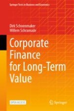
But there are also real options on E and S themselves, i.e. with the payoffs in terms of E and S, and possibly the underlying values as well. For example, a company’s activities might engender the option to improve or worsen biodiversity. And often, there is interaction between F options and S or E options, which can come at each other’s expense. In fact, companies are short a lot of options against society, but awareness of it is low. An airline can, for example, save on the maintenance of its airplanes. Against the annual cost savings, the airline creates a contingent liability in the form of increased likelihood of an accident. These interactions between F, S, and E options call for an integrated view on options, or even integrated value expressed in real options, which helps make these options and their trade-offs more explicit. See Fig. 19.1 for a chapter overview.
An illustration of the chapter overview consists of sustainability unaware, E S G integrated or inward view, impact or outward view, and integrated value.
Fig. 19.1
Chapter overview
×
Learning Objectives
After you have studied this chapter, you should be able to:
Demonstrate the basics of financial options.
Recognise and analyse real options.
Indicate how E and S can affect F options.
Take an integrated value perspective on a company, expressed as a set of options.
Advertisement
19.1 Financial Options
Financial options are option contracts that give their owners the right to sell or buy a security from the writer of the contract at a specified price. That specified price is the exercise price or strike price. The two parties to the contract have opposite positions: the buyer (owner) is long the option and has a right (not the obligation) to buy or sell; and the seller (the party who writes the contract) is short and has the obligation to fulfil the contract, if the buyer decides to enforce the contract and exercise their right to buy or sell. The owner pays a price for the option to the seller, known as an option premium.
Box 19.1 A Very Short History of Option Contracts
The first option contract on record was set up by the Greek philosopher Thales of Miletus around 600 BC. Expecting a strong olive harvest in the coming summer, Thales bought the right to rent all olive presses in the vicinity (a call option). When summer came, there was a heavy demand for olive presses and Thales exercised his right to rent cheaply. Having cornered the market, he could rent out the olive presses at high prices to become rich overnight.
Option contracts became a regular part of financial markets much later. Contracts with option features were used on the Antwerp bourse in the sixteenth century. And in the seventeenth-century Amsterdam, options on tulip bulbs were an important part of the tulip mania of the 1630s and the subsequent collapse of the Dutch economy. This gave options contracts their reputation as a speculative investment. Admittedly, it is hard to distinguish from the outside if investors use options for hedging or for speculation—the latter tends to be the case if the option is not combined with exposure to the underlying asset. This is especially risky when writing options without owning the underlying asset.
Option markets really took off in the 1970s with opening of the Chicago Board Options Exchange and the development of formal option pricing models. Hitherto, option pricing had been based purely on intuition. But even with formal option pricing models, disasters continue to happen. In fact, one could argue that the academic models gave a false sense of security, resulting in hubris on the part of their users. For example, in 1998, the hedge fund Long-Term Capital Management went bust in dramatic fashion due to events that were not even possible according to their models. This was all the more dramatic since it was run by, amongst others, Myron Scholes and Robert Merton, the Nobel prize winners and inventors of the Merton-Scholes option pricing model. This should have been a warning, but in the financial crisis of 2008–2009 too, options (and other contingent claims like credit default swaps) were a large part of the problem.
Options come in two main types: calls and puts. A call option gives the owner the right to buy a security, whereas a put option gives the owner the right to sell a security. The underlying security can be anything, such as a company’s stock, an exchange rate, or a commodity. Another distinction is between the so-called American and European options (so-called because both types are used globally): American options allow the owner to exercise the option at any time, whereas European options can only be exercised at the expiration date. This typically makes a European option less valuable than an American option with otherwise same terms.
19.1.1 Call Option: Long
Let’s consider the example of a call option on a bushel of wheat, with an exercise price of $10. Figure 19.2 shows the payoff structure at maturity of this call option.
A line graph of the pay-off versus the underlying value of the price of a bushel of wheat. The line is flat till (10, 0) and follows an increasing trend up to (20, 10). Data are estimated.
Fig. 19.2
Payoff structure of a call option on a bushel of wheat, excluding the premium
×
The underlying value is the price of a bushel of wheat. The exercise price of $10 means that the payoff is $0 for every price (of a bushel of wheat) below $10. For every price above $10, the payoff is the price minus the exercise price. So, at $10.70, the payoff is $10.70–$10 = $0.70.
The formula for the value of a long position in a call at expiration is:
$$ C=\max \left(S-K,0\right) $$
(19.1)
With S = the underlying value, and K = strike or exercise price.
At the time of writing in October 2022, wheat was traded for $9.66 per bushel. And it was about $12 at the start of the Russian invasion of Ukraine in February 2022. We can use these prices to see what the payoff would be. At a price of $9.66 per bushel, C = max(S−K,0) = max($9.66–$10,$0) = 0, if the option were to expire at that point in time. As the price of the underlying value is below the strike price, the call is said to be out-of-the-money. However, that does not mean that the value of the call is 0, unless it is at expiration. The longer the maturity of the call, ceteris paribus, the higher the probability that the underlying value will at some time exceed the strike price (and be in-the-money), and the higher its value. And since it has value, investors will be willing to pay a price for it, called a premium (which in a well-functioning market equals the consensus view).
Let’s suppose the premium that the owner has paid is $0.40 (we’ll get back to the drivers of that premium later on). Then the profit net of the premium is as follows: C-premium = max(S-K-premium,-premium) = max($9.66–$10-$0.4,-$0.4) = −$0.4. The payoff structure in Fig. 19.2 does not include the premium paid, but the profit diagram in Fig. 19.3 does include the premium.
A line graph of the profit versus the underlying value of wheat price. The line is flat till (10, minus 0.5) and follows an increasing trend up to (20, 9.5). Data are estimated.
Fig. 19.3
Profit diagram of a call option on a bushel of wheat, including the premium
×
Note that the payoff line has shifted below 0, and the break-even point is now at $10.40, where the underlying value equals the sum of the exercise price and the premium. Note that this does not mean that premiums are fixed: they move with the price of the underlying security. However, the buyer pays the premium to the seller at the time both parties enter into the contract, at which time the premium payment is fixed.
At a price per bushel of $10, the price of the underlying value exactly equals the strike price. The call option is then said to be at-the-money. C = max(S-K,0) = max($10–$10,$0) = $0 (this is the intrinsic value of the option without the premium). But again, before maturity the call option’s value will be positive to reflect the probability that it will be in-the-money later on. At a price of $12, C = max(S-K,0) = max($12–$10,$0) = $2. The option has a positive probability of ending up well in-the-money.
19.1.2 Call Option: Short
All of the above represent the perspective of the owner of the call, who has a long position. The seller, who writes the call, has the exact opposite payoff profile, as shown in Fig. 19.4. The payoff diagram shows that the losses can become very large when the wheat price increases.
A line graph of the pay-off versus the underlying value of the wheat price. The line is flat till (10, 0) and follows a decreasing trend up to (20, minus 10). Data are estimated.
Fig. 19.4
Payoff structure of a written call option on a bushel of wheat, excluding the premium
×
The payoff of the written call at expiration can be expressed as follows:
$$ -C=-\max \left(S-K,0\right) $$
(19.2)
At a price per bushel of $9.66, there is no payoff, since the price is below the strike price: -C = -max($9.66–$10,$0) = $0. But at a price of $12, the call is in-the-money, and negative value for the writer of the option: -C = -max($12–$10,$0) = −$2. Again, this is without the premium paid. Since this is the same contract as the long call example, we should use the same $0.40 premium. But now it works the other way: the writer of the call receives the premium as a compensation for writing the call. Hence, the line that is flat below the exercise price moves from $0 to $0.4 in Fig. 19.5.
A line graph of the profit versus the underlying value of wheat price. The line is flat till (10, 0.5) and follows a decreasing trend up to (20, minus 9.5). Data are estimated.
Fig. 19.5
Profit diagram of a written call option on a bushel of wheat, including the premium
×
Example 19.1 provides a problem to get familiar with calculating the value of a call option with premium.
Example 19.1 Calculating the Value of a Call Option with Premium
Problem
Investors expect share prices for Tech companies to rise in the next 6 months, so they decide to purchase a 6-month call option for an ETF (Exchange-Traded Fund) covering the biggest Tech companies. This ETF is worth $80 today, the strike price for the call option is $90 and the premium for this call option is $5. What is the value and net profit of the call option if the ETF is worth $80, $100, or $120 in 6 months? And at what ETF price does the call option break even?
Solution
Using Eq. (19.1), the value of the call option at an ETF price of $80 is C = max (S − K, 0) = max ($80 − $90, $0) = $0 and the net profit is $0 − $5 = − $5. At $100, the value of the call option is max($100 − $90, $0) = $10 and net profit is $10 − $5 = $5. At $120, the value of the call option is max($120 − $90, $0) = $30 and net profit is $30 − $5 = $25.
The call option breaks even when the value of the call option equals the option premium, thus max(S − $90, $0)= $5 which leads to an underlying value S of $95.
19.1.3 Put Option: Long
As mentioned above, a put option gives the owner the right to sell a security. Let’s again consider the example of an option on a bushel of wheat, again with an exercise price of $10. But this time it’s a put instead of a call. Figure 19.6 shows the payoff structure of this wheat put option for its owner.
A line graph of the pay-off versus the underlying value of wheat price. The line follows a decreasing trend from (0, 10) to (10, 0) and remains flat till (20, 0). Data are estimated.
Fig. 19.6
Payoff structure of a put option on a bushel of wheat, excluding the premium
×
The formula for the value of a long position in a put at expiration is:
$$ P=\max \left(K-S,0\right) $$
(19.3)
The exercise price of $10 means that the payoff is $0 for every price (of a bushel of wheat) above $10. For every price below $10, the payoff is the exercise price minus the price of wheat. So, at a wheat price of $4, the payoff is $10–$4 = $6.
As in the case of a call, a premium is paid. But we will skip discussion of the put premium here.
19.1.4 Put Option: Short
The seller, who writes the put, has the exact opposite payoff profile versus that of the buyer. This is shown in Fig. 19.7. At outcomes below the exercise price, the seller makes a loss, which can become quite significant at high volumes (i.e., many puts written) and at lower wheat prices (i.e., a bigger gap between price and exercise price to cover). Such losses may be neutralised by offsetting underlying positions, as we will see in the combined exposures below. But the losses can be dramatic in case of uncovered puts, i.e. without offsetting underlying exposures. The losses can be even worse for short calls. Figure 19.5 shows that these losses are not limited. For short put options, the downside is limited to the exercise price (which the writer has to pay to the owner of the put option).
A line graph of the pay-off versus the underlying value of wheat price. The line follows an increasing trend from (0, minus 10) to (10, 0) and remains flat till (20, 0). Data are estimated.
Fig. 19.7
Payoff structure of a written put option on a bushel of wheat, excluding the premium
×
The payoff of the written put at expiration can be expressed as follows:
$$ -P=-\max \left(K-S,0\right) $$
(19.4)
At a price per bushel of $9.66, the payoff is −$0.34 at maturity: -P = -max($10–$9.66,$0) = −$0.34. But at a price of $12, the put is out-of-money, and there is no payoff for the writer of the option: -P = -max($10–$12, $0) = $0. Example 19.2 provides an exercise for the valuation of a short put option.
Example 19.2 Calculating the Value of a Short Put Option
Problem
A commodity trader is confident that oil prices will continue to rise in the following 3 months and therefore decides to write 3-month put options for oil. The current price is $30 per barrel of oil, and the trader sets the strike price at $25 with a premium of $2.50. What is the value and net profit of the trader when the oil price reaches $20, $25, or $30 in 3 months? And below what price will the trader make a loss?
Solution
Using Eq. (19.4), the payoff for the writer of the short put option at an oil price of $20 is −P = − max (K − S, 0) = − max ($25 − $20, $0) = − $5. The oil trader is the writer of the option and thus receives the premium for the option. The trader’s profit is −$5 + $2.50 = − $2.50. The payoff at $25 is − max ($25 − $25, $0) = $0 and the profit is $0 + $2.50 = $2.50. At $30, the payoff is − max ($25 − $30, $0) = $0 and the profit is $0 + $2.50 = $2.50.
The trader will break even when − max ($25 − S, $0) = − $2.50 (the loss on the written put option equals the received premium), so at an oil price S of $22.50. When the oil price drops below $22.50, the trader will make a loss.
19.1.5 Combinations of Options & Hedging
The above payoffs were on a stand-alone basis, but in practice people can have composite exposures. And they may use options to hedge their exposures. Hedging is a strategy that tries to limit financial risk. For example, a farmer who has an upcoming wheat harvest will have a profit that depends on the wheat price, such as shown on the left-hand side of Fig. 19.8: since his costs are $5 per bushel, his profit per bushel will equal the wheat price minus $5. At any price below $5 he will be making a loss. However, by buying the put option described in Fig. 19.6 with an exercise price of $10, the farmer gets protection against potential losses. His payoff is his profitability before hedging (S-$5) plus the put’s payoff (max[K-S,0]) minus the put’s premium, so: (S-$5) + max($10-S,0)-$0.4. This means he obtains a profit of $4.6 at all wheat prices below $10. You can check the profit of $4.6: the farmer receives $10 as exercise price, has a cost of $5, and pays a premium of $0.4. Only if the wheat price goes above $10, does his profit rise proportionately with the wheat price, but he will still be making $0.4 per bushel less than in the case without hedging. This looks like a great deal: the put offers full protection on the downside against limited cost on the upside. So perhaps, the option is too cheap at $0.40? That depends on the chance of the wheat price ending up below $10.
3 line graphs of the pay-off versus the underlying value of wheat price. The graphs illustrate the profit of farmers before hedging plus the put option equals the profit of farmers after hedging. The lines of the profit of farmers before and after hedging follow an increasing trend.
Fig. 19.8
Farmer profit before and after hedging with a put
×
Whether to buy the put, and with what strike price, is not the only decision to make. The farmer also needs to decide on the volume: how many bushels does he expect to harvest? And for how many does he need protection?
A producer of packaged food faces an (almost) opposite exposure. The price per bushel hurts its profits since the food company needs to buy wheat for its production: profit per bushel is $17-S. Therefore, it might want to buy a call to protect against price rises. Figure 19.9 describes the company’s exposures before and after adding the call. As a result of this protection, the company’s payoff is now its original profit formula ($17-S) plus the call including its premium (max[S-$10,$0]-$0.4). So, for example, at a wheat price of $4 per bushel, its payoff is ($17–$4) + (max[$4–$10,$0]-$0.4) = $13 + $0–$0.4 = $12.6. And at wheat prices of $10 and higher, its profits are locked in at $6.60: all the losses on the original profit formula are offset by equal gains on the call. Note however that just like for the farmer, the company’s full exposure is not this simple, since it will also be determined by its production volumes—which are probably more predictable than the farmer’s harvest. Hence, for a full analysis, one should not only look at payoffs per unit (the price component), but at total payoffs including units (price times volume).
3 line graphs of the pay-off versus the underlying value of wheat price. The graphs illustrate the co-profit of food before hedging plus the call option equals the co-profit of food after hedging. The lines of the co-profit of food before and after hedging follow a decreasing trend.
Fig. 19.9
A food production company’s profit before and after hedging with a call
×
Example 19.3 provides an example of a steelmaker who hedges the price of iron. Iron is an important input to the steelmaker’s production process and the iron price can fluctuate.
Example 19.3 Calculating the Profit of a Steelmaker After Hedging
Problem
A manufacturer of steel products needs to buy iron as inputs for its production process and wants to protect itself from rising iron prices by buying a call option. The steelmaker’s profit formula is: $50-S, where S is the price of iron, and the call option uses a strike price of $20 with a premium of $4. What is the steelmaker’s profit when the price of iron is $10? And what is the maximum profit the steelmaker can earn when the iron price exceeds the strike price?
Solution
Using the steelmaker’s profit formula in combination with the long call formula (Eq. 19.1), the steelmaker’s profit is ($50 − S) + max (S − K, $0) − premium = ($50 − $10) + max ($10 − $20, $0) − $4 = $40 + $0 − $4 = $36.
The maximum profit the steelmaker can earn when the iron price equals or exceeds the strike price (S = K = $20) is ($50 − $20) + max ($20 − $20, $0) − $4 = $30 + $0 − $4 = $26. To check this you can use the situation where the iron price is higher, for example $40, and calculate the profit: ($50 − $40) + max ($40 − $20, $0) − $4 = $10 + $20 − $4 = $26. So, the maximum profit for the steelmaker is $26 when S ≥ $20.
19.1.6 Put-Call Parity
If you take another look at Figs. 19.8 and 19.9, you might notice that the farmer’s resulting exposure (third graph in Fig. 19.8) looks a lot like the call option used by the producer (second graph in Fig. 19.9), but simply at a higher level. And likewise, the producer’s resulting exposure (third graph in Fig. 19.9) looks very much like the put option used by the farmer (second graph in Fig. 19.8), but again at a higher level. In fact, one could argue that the farmer’s payoff on the portfolio containing the underlying value (in this case wheat) plus a put is essentially a call plus a bond (riskless debt with a fixed payoff) and that the company’s payoff on the portfolio containing a negative exposure to the underlying value and a call is a put plus a bond. Please note that the size of the bond equals the present value of the exercise price: B = PV(K). This was $10 in Figs. 19.8 and 19.9. One can make different combinations to arrive at the same result. This can be expressed in put-call parity:
$$ S+P=B+C $$
(19.5)
That is, the combined payoffs of the underlying value S and the put P are equal to the combined payoffs of a bond B and a call C. Figure 19.10 visualises these relationships.
5 line graphs of the pay-off versus the underlying value. They illustrate graph S plus graph P and graph B plus graph C equals graph S plus P equals B plus C. The line of graph S plus P equals B plus C follows an increasing trend.
Fig. 19.10
Put-call parity expressed in payoff structures
×
19.1.7 Capital Structure Expressed in Options
One can view capital structure (Chap. 15) in terms of options as well. As we will show, equity can be seen as a call option on the company’s assets (Merton, 1974); and corporate debt is effectively riskless debt minus a put on the company’s assets.
Equity as a Call Option on the Company’s Assets
Let’s take the market balance sheet of Table 19.1 as an example.
Table 19.1
Market value balance sheet
A table has the following values. In the first column, N P V of projects 20 and total assets 20. In the second column, debt 5, equity 15, and total liabilities 20.
The above values are given as static numbers, but in reality they can fluctuate over time as expected cash flows and/or discount rates change and affect the NPV of projects (estimated at market value). The NPV of projects is the driver of the value of assets and the value of equity. If the NPV of projects falls below 5, equity value goes to 0. For all values above 5, the value of equity moves proportionately with the NPV of projects. Therefore, one can regard the equity as a call option on the company’s assets, whereby the exercise price is the face value of debt1 (in this case 5). See Fig. 19.11.
A line graph of the pay-off to equity versus the underlying value of company value. The line follows an increasing trend from (5, 0) to (35, 30). The value of equity is at (20, 15). Data are estimated.
Fig. 19.11
Equity value expressed as a call option on company value
×
Remember the formula for the value of a call option at maturity:
Thinking in terms of options provides a dynamic perspective on value, recognising that the current value of equity may be 15, but that the leverage means that the equity value is extra sensitive to changes in asset value. Figure 19.11 shows that the equity holders (stockholders) get the full potential of the upside and have limited their losses on the downside (they can at most lose their invested capital of 15 due to limited liability). Equity holders thus favour risky projects with an equal up- and downside risk profile. Volatility of the underlying value (in this case the company’s assets) increases the value of a call option (see Fig. 19.22 on drivers of option prices below).
Corporate Debt as Riskless Debt Minus a Put on the Company’s Assets
Now that we know that equity can be expressed in options, it follows from put-call parity that corporate debt can also be expressed in terms of options. After all from Eq. 19.5, we have:
$$ S+P=B+C $$
(19.8)
where S = assets; P = put on assets; B = riskless debt; C = call on assets. Hence, assets can be expressed as:
$$ Assets=S=B-P+C $$
(19.9)
Figure 19.12 illustrates this relationship. Assets is equal to riskless debt minus a put option on assets plus a call option on assets.
4 line graphs of the pay-off versus the underlying value of assets. They illustrate graph S plus equals graph B plus graph minus P plus graph C. The line of graph S follows an increasing trend.
Fig. 19.12
Assets expressed in put-call parity terms
×
From Chap. 15 on capital structure, we know that assets are financed by equity and debt. This company debt is risky, because a company can fail. Assets can thus be expressed as follows:
$$ Assets= Risky\ debt+ Equity $$
(19.10)
where from Eq. (19.7), we can express equity as follows:
$$ Equity=C $$
(19.11)
Rewriting Eq. (19.10), we can derive risky debt as follows:
Equation 19.12 implies that risky debt is essentially riskless debt minus a put on assets, i.e. riskless debt plus a written put on the company’s assets (remember a written put is a short position in a put). Figure 19.13 illustrates the payoff structure of risky debt. Again, the value of the put option increases with volatility of the company’s assets (Fig. 19.22 below). So debt holders try to avoid risk, whereas equity holders love risk to a certain extent. Banks and bondholders therefore use loan and bond covenants, which restrict the company’s ability to take on risk.
A multiple-line graph of the pay-off to equity versus the underlying value of company value plots the risky debt, riskless debt, and written put. The lines of risky and riskless debt are flat at the pay-off 5 and the line of written put is flat at the pay-off 0. Data are estimated.
Fig. 19.13
Risky-debt value expressed as riskless debt minus a put on company value
×
Example 19.4 asks you to calculate the value of risky debt.
Example 19.4 Calculating the Value of Risky Debt
Problem
The market value of Pharma’s assets is $100 million. The face value of its debt is $40 million. A put option on Pharma’s assets with a strike price of $40 million trades at $0.5 million. What is the current value of Pharma’s risky debt? And what is the value of Pharma’s equity?
Solution
The face value of debt is the nominal value of debt. It represents the value of riskless debt B (with no default risk). Using Eq. (19.12), the value of Pharma’s risky debt is B − P = $40 − $0.5 = $39.5 million. Next, using Eq. (19.10), the value of Pharma’s equity is Equity = Assets − Risky debt = $100 − $39.5 = $60.5 million.
The written put is worth $0.5 million. This amount is added to the equity holders’ value at the expense of bondholders.
19.1.8 Option Quotations
Options are most commonly traded on stocks. 3M is a US conglomerate company that is well known for its Post-It and Scotch Tape products. Table 19.2 gives quotations for options on 3M stock with expiration in January 2025, priced as of Mid-October 2022, when the price of the stock was $113.49. Table 19.2 shows three strike prices (in reality, many more are available): one much below the stock price, one very close to the stock price, and one much above the stock price. We need some terminology to understand the option quotations in Table 19.2:
The strike price of an option is a fixed price at which the owner of the option can buy (in the case of a call), or sell (in the case of a put), the underlying security (or commodity);
The bid price is the price at which market makers (see Box 8.2 on the role of market makers) are willing to buy the option;
The ask price is the price at which market makers are willing to sell the option;
Open interest refers to the number of options or future contracts that are held by traders and investors in active positions. These positions have been opened, but have not been closed out, expired, or exercised.
Table 19.2
Quotations for options on 3M stock, per October 2022 with expiration in January 2025
Strike*
C or P
Bid*
Ask*
Open interest
60
C
53.50
55.55
0
P
2.97
3.90
20
110
C
20.50
21.75
17
P
16.90
18.00
64
160
C
5.65
6.45
25
P
49.15
50.70
2
Notes: *Prices in US dollar. The current stock price is $113.49
With a strike price of $60, the call is very much in-the-money. The payoff would be: C = max [S − K, $0] = $113.45 − $60 = $53.45, if the option on 3M stock were exercised today. This is called the intrinsic value of the call option (see Fig. 19.14). The option premium—the average of bid and ask—is $54.52, which is $1.07 higher. This is called the time value of the call option. It is the amount an investor is willing to pay for an option above its intrinsic value and reflects hope that the option’s value increases before expiration due to a favourable change in 3M’s price (see Fig. 19.14).
A dual-line graph of value versus stock price plots the option values and the intrinsic values. Both the lines follow an increasing trend. The distance between the lines is the time value.
Fig. 19.14
Option value before expiration at time t
×
Conversely, at that strike price of $60, the put is very much out-of-the-money if 3M stock hits $110 at maturity, since max(K − S, 0) = max ($60 − $110, $0) = $0. Hence, the much lower option premium of $3.44 (=($2.97 + $3.90)/2) on the put than on the call. The put premium reflects only the time value, since the intrinsic value is zero for this particular put option.
At a strike price of $160, the reverse holds: the put is very much in-the-money (max[K − S, 0] = max [$160 − $110, $0) = $50), with a price around $50; and the call is out-of-the-money (max[$110 − $160, $0] = $0), and a price (or premium) around $6, reflecting a small but serious chance that 3M’s stock price goes over $160 in the next 3.25 years.
At a strike price of $110, there is only a small gap between the strike price and the share price of $3.45. However, the prices of the puts and calls are much higher, reflecting the possibility that the share price will go much higher or much lower than the strike price during the lifetimes of the options.
As discussed, Fig. 19.14 illustrates the option value (also called option premium or option price) as the sum of the intrinsic value and the time value:
$$ Option\ value= intrinsic\ value+ time\ value $$
(19.13)
Example 19.5 gives an exercise to calculate the value of stock options.
Example 19.5 Calculating the Value of Stock Options
Problem
The price of the S&P 500 Index in March 2023 is around $4000. The quotations for options on S&P 500 Index stock, per March 2023, with expiration in December 2025, are given in the table below. Calculate the premium, the intrinsic value, and the time value of each call and put option for the given strike price.
Strike
C or P
Bid
Ask
3600
C
882.10
942.40
P
266.90
281.90
3800
C
776.90
800.60
P
320.10
336.60
4000
C
657.90
682.40
P
380.20
397.30
4200
C
547.00
569.30
P
447.60
471.82
4400
C
443.80
466.70
P
523.10
542.00
Solution
The option premium (or option value) is the average of the bid and the ask. The price of the S&P Index is S = $4,000. The premium, the intrinsic value, and the time value of each call and put option are calculated in the table below. The time value is relatively large, which reflects the long maturity (2 years and 9 months) of the options and the volatility of the S&P index.
Strike (K)
C or P
Premium
Intrinsic value
Time value
Calculation
(Bid + Ask)/2
C = max (S − K, 0)
P = max (K − S, 0)
Premium – Intrinsic value
3600
C
912.25
400
512.25
P
274.4
0
274.4
3800
C
788.75
200
588.75
P
328.35
0
328.35
4000
C
670.15
0
670.15
P
388.75
0
388.75
4200
C
558.15
0
558.15
P
459.71
200
259.71
4400
C
455.25
0
455.25
P
532.55
400
132.55
19.2 Valuing Options
So far, we have described what the payoffs of certain options are. The non-linear nature of these payoffs makes valuation of options difficult. The standard discounted cash flow (DCF) model is difficult to use. But models have been developed that derive the value of an option.
Options are priced using no-arbitrage principles. This is most easily explained using the put-call parity (static arbitrage), introduced in Sect. 19.1. In order to use the put-call parity, you need a correctly priced put to price a call, and that is not always available. Therefore, we need to resort to a different approach that uses a dynamic trading strategy over multiple periods. The idea is still the same. We design a trading strategy that exactly replicates the option payoffs. This strategy should be self-financing such that we do not need to add or withdraw money at intermediate time points. This way, we can price the option at time 0 as the required starting capital for this dynamic trading strategy. The dynamic trading strategy is used in the binomial option pricing model, which can be extended to the well-known Black-Scholes option pricing model.
19.2.1 The Binomial Option Pricing Model
The binomial option pricing model (Cox et al., 1979; Rendleman, 1979) prices options by making the simplistic assumption that at the end of the next period, the underlying value has only two possible values. The two-state single period model values a call option by building a replicating portfolio, which is a portfolio of other securities that has the same value as the option in one period. As they have the same payoffs, the law of one price (see Box 4.1) tells us that the call and the replicating portfolio of stocks and bonds should have the same value.
A Call in the Binomial Model
The example in Fig. 19.15 shows how that works in a binomial tree, a timeline with two branches per date that show alternative possible events. The starting point is a call with a strike price of K = $10 on a stock with a value of S = $10. The decision tree shows two possible values for the stock in the next period: Su = $12 in the up state u, and Sd = $8 in the down state d. This results in values for the call of Cu = $2 in the up state and Cd = $0 in the down state. During the same period, the riskless bond B gives a return of rf = 3%.
A binomial tree illustration of stock and bond of $10 and $1 is classified into up and down. The up values are as follows. Stock $12, Bond $1.03, and Call $2. The down values are as follows. Stock $8, Bond $1.03, and Call $0.
Fig. 19.15
Binomial tree for a call
×
The question then is: how to replicate the call with (parts of) a stock and (parts of) a bond? The idea is to buy stock in such proportions that they give exactly the same payoffs as the call, i.e. $2 in the up state and $0 in the down state. The bought stock (long position) is financed by selling bonds (short position). The first step is to determine the option delta (or hedge ratio), which is the number of stocks needed to replicate or hedge the call. The option delta Δ is defined as follows:
The intuition of Eq. 19.14 is as follows. One is ‘hedged’, when the following identity holds at t = 1: Δ x spread of possible stock prices = spread of possible option prices. In our example of Fig. 19.15, the option delta is \( \Delta =\frac{\$2-\$0}{\$12-\$8}=0.5 \).
The second step is to determine the number of bonds needed to finance the stock position. We are working with a replicating portfolio, which means that the payoff on the stocks and bonds replicates the payoff on the call option. This replication, for one time period later, is for the up state Cu = Δ ∙ Su − (1 + rf) ∙ B, and for the down state Cd = Δ ∙ Sd − (1 + rf) ∙ B. Note that we have to increase the bonds with the paid interest rf over one period. A single bond is valued at B = $1 in Fig. 19.15. Rearranging, we can derive the number of bonds B:
Filling in, we get for the up state B = (0.5 ∙ $12 − $2)/1.03 = $3.8835. As the replication should work in the same way for the two states, we can check for the down state B = (Δ ∙ Sd − Cd)/(1 + rf) = (0.5 ∙ $8 − $0)/1.03 = $3.8835. They are the same!
The final step is to determine the price of the call. Again, we can use the replicating portfolio. The price of the call option in the binomial model is as follows:
Now, we are ready to calculate the value of the call option today, using the stock price S and bond price B at t = 0, one period before the final payoff at t = 1. Using Eq. 19.16, we get C = 0.5 ∙ $10 − $3.8835 = $1.1165.
Table 19.3 provides a final check that the no-arbitrage principles work. At each point in time (t = 0 and t = 1) and for each scenario (up and down), the value of the replicating portfolio equals the value of the call.
Table 19.3
Call equals replicating portfolio in each scenario
Instrument
Period t = 0
Period t = 1
Up
Down
Replicating portfolio
Δ ∙ S − B=
0.5*$10 - $3.8835 =
$1.1165
Δ ∙ Su − (1 + rf) ∙ B=
0.5*$12 – (1.03)*$3.8835 =
$6 - $4 = $2
Δ ∙ Sd − (1 + rf) ∙ B=
0.5*$8 – (1.03)*$3.8835 =
$4 - $4 = $0
Call
C = $1.1165
C = $2
C = $0
A Put in the Binomial Model
The calculation of the put price occurs in a similar way. The starting point is a put with similar prices: a strike price of K = $10 on a stock with a value of S = $10. The decision tree in Fig. 19.16 is similar to Fig. 19.15, except for the put: the values for the put of Pu = $0 in the up state and Pd = $2 in the down state.
A binomial tree illustration of stock and bond of $10 and $1 is classified into up and down. The up values are as follows. Stock $12, Bond $1.03, and Put $0. The down values are as follows. Stock $8, Bond $1.03, and Put $2.
Fig. 19.16
Binomial tree for a put
×
Building on Eq. 19.14, the option delta Δ is defined as follows:
Whereas one needs a positive number of stocks to hedge a call option (the stock and call option both increase with a rising stock price), the option delta is negative for a put (the put option decreases with a rising stock price). So, in our example of Fig. 19.16, the option delta is \( \Delta =\frac{\$0-\$2}{\$12-\$8}=-0.5 \), which means that one has to sell stocks to hedge a put option. The replicating portfolio has thus a short position in stocks and a long position in bonds. This replication is for the up state Pu = Δ ∙ Su + (1 + rf) ∙ B and for the down state Pd = Δ ∙ Sd + (1 + rf) ∙ B. Rearranging these equations, the number of bonds B is:
Filling in, we get for the up state B = (−(−0.5) ∙ $12 + $0)/1.03 = $5.8252. We leave it to the reader to check that the number of bonds is the same for the down state. The price of the put option in the binomial model is as follows:
We can calculate the value of the put: P = − 0.5 ∙ $10 + $5.8252 = $0.8252. We are now able to calculate the value of a call option and that of a put option with the binomial option pricing model. Box 19.2 checks our calculations with the put-call parity. Next, Example 19.6 gives you the opportunity to calculate the value of a call option with the binomial model.
Box 19.2 Put-Call Parity in the Binomial Pricing Model
We can use put-call parity to check the calculations for the prices of the call and put options in Figs. 19.15 and 19.16. The put-call parity from Eq. 19.5 is:
$$ S+P= PV(K)+C $$
We can check the put-call parity directly by putting the relevant prices in: $10 + $0.8252 = ($10/1.03) + $1.1165 = $10.8252. It holds!
We can also check the formula in an analytical way. Filling in the put and call option formulas of Eqs. 19.19 and 19.16, we get: S + Δp ∙ S + Bp = PV(K) + Δc ∙ S − Bc. Rearranging, we obtain: S + Bp + Bc = (Δc − Δp) ∙ S + PV(K). This means for the stocks that 1 = (Δc − Δp). This holds in our example: 0.5 − − 0.5 = 1. Next, for the bonds: Bp + Bc = PV(K). Again, this holds $5.8252 + $3.8835 = $10/1.03 = $9.7087.
Example 19.6 Calculating the Value of a Call Option with the Binomial Model
Problem
A stock has a current value of $40 and two possible values for the next period, namely $36 and $46. In addition, the risk-free rate equals 2%. What is the value of a call option calculated using the binomial model?
Solution
To calculate the value of the call option, you first need to determine the delta and number of bonds. The delta is calculated using Eq. 19.14. In this case, the delta is \( \Delta =\frac{C_u-{C}_d}{S_u-{S}_d}=\frac{\$6-\$0}{\$46-\$36}=0.6 \). The number of bonds is calculated using Eq. 19.15. We first calculate the up-state values as follows: \( B=\frac{\Delta \bullet {S}_u-{C}_u}{1+{r}_f}=\frac{0.6\bullet \$46-\$6}{1.02}=\$21.18 \). Next, we calculate the down-state values: \( B=\frac{\Delta \bullet {S}_d-{C}_d}{1+{r}_f}=\frac{0.6\bullet \$36-\$0}{1.02}=\$21.18 \), which is the same as for the up-state values. Lastly, the value of the call option can be determined using Eq. 19.16: C = Δ ∙ S − B = 0.6 ∙ $40 − $21.18 = $2.82.
19.2.2 Multiperiod Binomial Model
The formula for the option delta Δ can be interpreted as the sensitivity of the option’s value to changes in the stock price at each point in time. Let’s expand our one period binomial tree in Fig. 19.15 for a call to a two-period binomial tree. Figure 19.17 shows that in the up state at $12 at t = 1, the stock can go up again to $14 in t = 2. It can also go down to $10. In the down state at $8 at t = 1, the stock can go up to $10 at t − 2 (the same as the down movement of the up state) or go down to $6.
A 2-period binomial tree illustration of stock of $10 is classified into up and down of $12 and $8 respectively. The up value is classified into up and down of $14 and $10. The down value is classified into up and down of $10 and $6.
Fig. 19.17
Two-period binomial tree for a call
×
We can value the call option in the multiperiod binomial tree by working backwards from the end at t = 2. Let’s start with the situation that the stock price has gone up to $12 at t = 1. Figure 19.18 shows the payoffs for the stock and the call. Remember that the exercise price of the call is $10. This results in values for the call of Cu = $4 in the up state with a stock price of Su = $14, and Cd = $0 in the down state with a stock price of Sd = $10. Using eq. 19.14, we can calculate the delta Δ:
A binomial tree illustration of a stock of $12 is classified as up and down. The up values are stock $14 and call $4. The down values are stock $10 and call $0.
So, the value of the call option in the up state at t = 1 is $2.291.
We can repeat the same exercise for the down state. Figure 19.19 shows that the payoff on the call is $0 in the up and down state at t = 2. A call with zero payoffs in the future also has zero value today. So, the value of the call option in the down state at t = 1 is $0. To check this, we can also calculate the delta
A binomial tree illustration of a stock of $8 is classified as up and down. The up values are stock $10 and call $0. The down values are stock $6 and call $0.
The delta is also zero, so we need zero stocks to hedge this position.
The final step is calculating the value of the call option at t = 0 in Fig. 19.20. As discussed before, the option delta—which is the number of stocks needed to hedge the call option—has to be recalculated at each point in time when the stock or call data change. Although Fig. 19.20 and Fig. 19.15 look almost the same, there is a small difference. The payoff on the original call option in the one-period model in Fig. 19.15 is $2 at t = 1 and that on the new call option is $2.291 in the two-period model in Fig. 19.20 at t = 1. Using Eq. 19.14, the delta Δ is:
A binomial tree illustration of a stock of $10 is classified as up and down. The up values are stock $12 and call $2.291. The down values are stock $8 and call $0.
So, the value of the call option at t = 0 is $1.279, which is slightly higher than the one-period call with a value of $1.1165.
We can refine the tree by cutting the maturity of the call option in ever smaller increments. As a result, the return distribution at t = T (maturity) starts to approximate the real returns distribution ever better. There is also the limiting case in which the time to maturity is cut off into infinitely many increments that are each infinitely small. This gives the Black-Scholes option pricing model, which is in continuous time.
19.2.3 The Black-Scholes Option Pricing Model
The Black-Scholes option pricing model (Black & Scholes, 1973) was developed independently and before the binomial model. But it is related to the binomial option pricing model and can be derived from it (see, for example, Hull, 2014). The Black-Scholes formula for the price of a European call on a non-dividend paying stock follows the set-up of the binominal model in Eq. 19.16:
PV(K) is the present value (and price) of a risk-free zero-coupon bond that pays K on the expiration date of the option discounted at the risk-free rate.
K is the exercise price.
N(d) is the cumulative normal probability distribution, i.e. the probability that a normally distributed variable is less than or equal to d
σ is annual volatility (standard deviation) of the stock’s returns.
T refers to the number of years until expiration.
Let’s discuss the features of the Black-Scholes formula. First, the stock price S plays an important role in option pricing. As stock prices cannot fall below zero, the left side of the stock price is limited. But stock prices can increase to very high numbers, though the chance of that happening is small. The lognormal function (denoted by ln in Eq. 19.20) is therefore used for the stock price.
The next step is to interpret the cumulative normal distribution N(d), which is illustrated in Fig. 19.21. This is the probability that a randomly distributed variable will be less than d: the shaded area left of d in Fig. 19.21. N(d1) is the option delta, which we introduced earlier. If d1 is large, then N(d1) is close to one. In economic terms, this means that the stock price S is large relative to the present value of the exercise price PV(K). The call option is then very much in-the-money and one needs almost a full stock to hedge the fluctuations of the call option (i.e. the option delta is close to one). If d1 is zero, then N(d1) is 0.5. Figure 19.21 shows that half of the probabilities are in that case to the left.
A frequency graph of the cumulative normal distribution. The line follows a bell-shaped trend with a probability peak of 0.40 approximately.
Fig. 19.21
Cumulative normal distribution
×
N(d2) is the normal distribution corresponding to the probability that the call option will be exercised at expiration (remember the Black-Scholes formulas are used for European call and put options, which can only be exercised at expiration). An easy way to calculate N(d) is to use the excel function NORMSDIST(d).
Finally, the volatility of the underlying stock σ is an essential variable of the Black-Scholes formula. Options are useful to protect or ‘hedge’ the owner of stocks against volatile stock prices, as discussed in Sect. 19.1. Without volatility in the underlying value, there is little use for options.
Example 19.7 calculates the value of the 3M call option with the Black-Scholes model.
Example 19.7 Calculating the Value of a Call Option with the Black-Scholes Model
Problem
We use the values of the 3M call option with exercise price of $110 from Table 19.2. Next, we take a given volatility of 25%, a risk-free rate of 2.5%, and 2.25 years to maturity. What is the option delta, the number of bonds needed and the value of the call option?
Solution
The value of the call can be determined using eq. 19.20. In order to fill in the complete formula, the option delta and the number of bonds need to be determined first. To determine the option delta, the present value of the exercise price is need. For the exercise price of $110, the present value is \( PV(K)=\frac{\$110}{(1.025)^{2.25}}=\$104.06 \).
The option delta is the normal distribution of d1, which leads to N(0.4189) = 0.662. The number of bonds is calculated by multiplying the normal distribution of d2 with the present value of the exercise price, so N(0.0439) ∙ $104.06 = 0.518 ∙ $104.06 = $53.85. Now that all the variables for the calculation of the call option are calculated, inserting them into Eq. 19.20 gives:
To check our calculation, we can compare the option value with the option premium in Table 19.2, which is \( \frac{\mathrm{bid}+\mathrm{ask}}{2}=\frac{\$20.50+\$21.75}{2}=\$21.13 \). This shows that our option value of $21.32 is close to the option premium of $21.13 quoted in the market.
Using the put-call parity from Eq. 19.5, we can show the put as follows:
$$ P=C-S+ PV(K) $$
(19.21)
We can now insert the Black-Scholes formula of Eq. 19.20 for the call C and rearrange. This gives us the Black-Scholes formula for the price of a European put on a non-dividend paying stock:
$$ P=\left[1-N\left({d}_2\right)\right]\bullet PV(K)-\left[1-N\left({d}_1\right)\right]\bullet S $$
(19.22)
Interestingly, only a very limited number of input parameters are needed to price the Black-Scholes call and put options. For example, we don’t need to know the expected return on the stock (which is already in the current stock price). In Sect. 19.2.4, we review the drivers on option prices.
Dividend Paying Stocks
The Black-Scholes formulas are derived for non-dividend paying stocks. They can easily be adjusted for dividend paying stocks. The European call option holder has no rights to any dividends paid out prior to expiration. We can just deduct the present value of these missed dividends PV(Div) from the stock price S:
$$ {S}^{\ast }=S- PV(Div) $$
(19.23)
The adjusted stock price S∗ in place of S can then be used in the Black-Scholes formulas.
Implied Volatility
While most parameters are easy to calculate, the volatility of the stock price σ is more difficult to calculate. The most direct way is to calculate a stock’s volatility from historical stock prices (see Chap. 12). But traders sometimes take a shortcut by deriving a stock’s volatility from the current market prices of traded options. By filling out all other parameters and the market price of the option, the volatility can be obtained. Estimating a stock’s volatility that is implied by an option’s market price is called implied volatility.
Risk of Options
What are the risks of options? We can derive the risk of an option from the underlying replicating portfolio. In the case of a call option, the portfolio is long in stocks and short in bonds. From Eq. 13.7 in Chap. 13, we know that the beta of the option βoption is a weighted average of the beta of the stock and the bond:
Given that the bond is risk-less, its beta is βbond = 0. Let’s calculate the beta of the 3M call option in Table 19.2. From Example 19.7, we know that Δ ∙ S = 0.662 * $113.49 = $75.13 and B = 0.518 * $104.06 = $53.85. Remember that for a call option, the delta ∆ is positive and the bond financing B is negative. 3M’s stock beta is β3M = 1. The beta of the option is βoption = ΔS/(ΔS + B) ∙ βstock = $75.13/($75.13 − $53.85) * 1 = 3.53. The beta of the 3M call option (3.53) is far higher than the beta of the stock (1) and thus riskier than the stock itself. This can be explained by the fact that a call option is basically a leveraged position in the stock, as the replicating portfolio finances the stock with borrowing.
Please note that the option beta βoption changes at each point in time. After all, you have a dynamic trading strategy in which delta Δ changes at each point in time. While the beta of a call is positive, the beta of a put is typically negative reflecting the short position in stocks.
19.2.4 Drivers of Option Prices
The Black-Scholes formulas reveal the drivers of option prices, which are summarised in Fig. 19.22.
A radial illustration lists 5 drivers of option prices. The drivers are the time to expire, risk-free interest rate, strike price, underlying value, and volatility.
Fig. 19.22
Drivers of option prices
×
Two out of these five drivers have the same sign for (long positions in) calls and puts: the time to expiration (+) and volatility (+). After all, the longer the option runs, and the higher its volatility, the bigger the chance that it will become in-the-money. The probability of really large swings increases, since there is little downside to a swing to one side and a lot of upside to the swing to the other side. Just imagine the reverse: an out-of-the-money call (or put) option with a very short time to expiration and a very low volatility—its price will likely be low.
The other three drivers have opposing signs for (long positions in) calls and puts, of which one has a negative sign for calls and a positive sign for puts: the strike price. The intuition on the strike price already followed from the discussion in Sect. 19.1: the higher the strike price, the lower the expected payoff on a call. This brings us to the two drivers that have positive signs for calls and negative signs for puts: the risk-free rate and the underlying value. The underlying value was already discussed in Sect. 19.1: the higher the underlying value, the higher the expected payoff on a call. And a higher risk-free rate lowers the PV of the strike (or exercise) price, which is positive for the call price and negative for the put price. Table 19.4 summarises the effect of drivers on call and put options.
Table 19.4
Effect of drivers on (long positions in) call and put options
Driver
Call option
Put option
Underlying value
+
−
Volatility
+
+
Strike price
−
+
Time to expiration
+
+
Risk-free interest rate
+
−
19.3 Real Options on F
A real option is the opportunity to make a particular business decision. In contrast to financial options, they are not exchange traded, and there is no formal option contract, and no clear counterparty. Otherwise, they have the same characteristics, namely with a payoff that depends on factors such as the underlying value and a strike price on that underlying value. Being long in real options provides valuable flexibility to exercise an opportunity, whereas being short in real options (which may happen unknowingly) can be very risky and value destructive.
This section discusses what real options look like, how they arise, and what they mean in terms of financial value. In subsequent sections, we discuss how E and S affect such real options on F (Sect. 19.4); real options on E and S themselves (Sect. 19.5); and how real options on E, F, and S relate to each other in integrated value (Sect. 19.5). We note at the outset that you typically cannot price real options by no-arbitrage principles as we did in the previous sections, since these real options are not redundant. This means you cannot make a replicating portfolio to price real options.
19.3.1 Applications of Real Options
Many corporate assets, particularly growth opportunities, can be viewed as call options (Myers, 1977). The value of such ‘real options’ depends on discretionary future investment by the firm. These options can be used in valuation and (corporate) investment decisions, including M&A. For example, suppose a company has developed a technology to make battery materials for electric vehicles that replaces polluting metals with lignin (wood). As almost always, the initial problem is the higher cost of the new technology versus existing alternatives. The company now effectively has a put option on the production costs of lignin-based battery materials (which need to go down to be competitive), where the exercise price is the production costs of traditional metals-based battery materials products (which are lower, but may rise). When the production costs of lignin-based battery materials go down, the put option comes in-the-money.
This is just one example, but there are many more. See Fig. 19.23 for a classification of more often occurring types. These options are very important for companies. In fact, one could argue that corporate strategy is all about options. As Luehrman (1998) puts it: ‘In financial terms, a business strategy is much more like a series of options than a series of static cash flows’. One could also view high risk companies as options, for example in a venture capital portfolio, where two-thirds of investments tend to lose money and most of the returns come from just a few blockbusters (see Chap. 10). Typical examples include biotech R&D investments, where most don’t pay off, but some pay off massively; and mining exploration, which gives the option to build a mine, and which is exercised if the price of the mined material is sufficiently high.
3 table illustrations. The real call options list option to defer, expand, extend, and increase scope. The real put options list abandonment option, the option to shrink and shorten. The combination lists follow switching options.
Fig. 19.23
Classification of real options
×
To stress the strategy angle, Box 19.3 shows how Shell created a put option to cancel refinery construction ahead of the oil crisis in the 1970s. This put option appeared to be very valuable when the oil crisis hit.
Box 19.3 Put option on Refinery Capacity
Oil company Shell is one of the first companies to do long-term scenario analysis (see Chap. 2). The business model of oil companies can be affected by several political and economic trends. Shell’s scenario analysis in the early 1970s showed the possibility of reduced oil supply from the Middle East. And importantly, Shell acted on this knowledge by putting a clause in its contracts with refinery constructors to delay or cancel the building of refineries. They could do this at negligible costs. When the oil crisis hit in the 1970s, Shell exercised this put option by cancelling the building of new refineries, as these would be idle given the reduced oil supply.
Shell saved a lot of money by exercising its put option, while other oil companies had to keep on building refinery capacity (without business for these refineries), since they did not have the flexibility to delay construction.
The lesson from this case study is that it is important to put scenario analysis into strategic action. Once a company becomes aware of undesirable scenario outcomes, it should act on it as part of its strategy to navigate away from these possible outcomes.
Koller et al. (2020) provide a classification of real options (see Fig. 19.23):
The option to defer (a call): the flexibility to wait and do the same action later (e.g., a product introduction), when conditions (the underlying value) are better;
The abandonment option (put): the option to stop an operation, for example to shut down a plant at a cost (the exercise price) to avoid much higher on-going costs (negative exposure to the underlying value);
The follow-on (compound) option (a series of options on options): for example, the ability to launch a new product, for which the experience of previous products is a prerequisite;
The option to expand (call) or contract (put): flexibility in the size of the operations, for example to operate a mine or factory at larger (call) or smaller (put) volumes per unit of time;
The option to extend (call) or shorten (put): the flexibility to adapt the lifetime of an operation, i.e. to operate for longer (call) or shorter (put);
The option to increase scope (call): the flexibility to add other operations, such as new products, new features, or new markets to existing operations;
Switching options (a portfolio of call and put options): flexibility to choose between different operations; for example, to increase the production of a product in high demand at the expense of another product that is less in demand.
The drivers of real options follow from the drivers of financial options and are summarised in Fig. 19.24. A key point is that uncertainty—measured as volatility of cash flows—enhances the flexibility value (though it may also reduce future cash flows). Real options are about creating flexibility to change course in future circumstances. In this future, the cash flows of the existing course of action (e.g. the incumbent product or technology) and/or the alternative course of action (e.g. a new product or technology) may change.
A radial illustration lists the factors that enhance flexibility value. The components are the time to expire, risk-free interest rate, investment costs, cash flows existing business, lost cash flows, underlying cash flows alternative, and uncertainty about C F.
Fig. 19.24
Drivers of real option value. Note: The drivers of a real call option are shown. Source: Adapted from Koller et al. (2020)
×
But these real options are typically not costless. Investment is often necessary to create the option and can thus be seen as a premium paid for the option. There may also be lost cash flows from an option to defer; the company could, for example, have increased sales today if it had not deferred the launch of a new product.
19.3.3 Real Options to Deal with Uncertainty
Companies can use real option analysis when faced with fundamental uncertainty, if not only the outcome, but also the probability distribution governing the outcome, is unknown. If the probability distribution is known, scenario analysis can be used (see Sect. 12.8 in Chap. 12). If the probability distribution is unknown, real options can be used to structure the challenge for the company and prepare decisions in the future.
Let’s illustrate this with an example. In the energy transition, it is not (yet) clear which renewable energy source (wind, solar or hydrogen) is the most profitable and will emerge as the ‘winning’ technology. A company can prepare itself by making (small) investments in the various technologies. The company is then ready for expansion when it becomes clear which type of renewable is the most profitable. The option premium is then the upfront investment and the real options are the option to expand (in the winning technology) and to switch (from the non-winning technologies). As shown below, real option analysis works backwards. It starts with possible outcomes (in our example, possible renewable technologies) and then defines the options in the intermediate period (choice to expand/switch) and at the start (decision to do initial investment).
19.3.4 Using Decision Tree Analysis for Real Options
Real options can be analysed using decision trees that are reminiscent of the multiperiod option pricing model. A decision tree is a graphical representation of future decisions under uncertainty. Figure 19.25 gives the example of a decision tree regarding the investment in a mine. A decision tree is different from a binomial tree, in which the branches of the tree represent uncertainty that cannot be controlled: the nodes are only information nodes (uncertainty out of control of the decision maker; in red in Fig. 19.25). A decision tree also has decision nodes (in blue in Fig. 19.25).
A decision tree illustration of cash classified into to invest and do not invest in a mine. Invest in a mine is followed by minus $2500 which is classified into metal prices rise of $5500 million and fall of $800 million.
Fig. 19.25
Decision tree example
×
The investment in the mine (a cash flow of -$2500 million) at t = 0 effectively buys the company an exposure to metal prices, with a payoff of $5500 million if prices rise; and a $800 million payoff if prices fall at t = 2. Note that the investment in the mine is NOT a call anymore at t = 1 once the mine has been built at t = 0. The call lies before that at t = 0: the choice to build it or not; and before that at t = − 1 (outside Fig. 19.25): the choice to do the exploration or not. Table 19.5 shows the (expected) payoffs and how they add up. Please note that Table 19.5 starts from the right side of the decision tree and then works backwards. Table 19.5 shows a total expected payoff of $650 million, suggesting that the company should invest in the mine. Example 19.8 shows how one can calculate the expected value with a decision tree.
Table 19.5
Expected value in the decision tree example ($ million)
Scenario
Payoff (1)
Probability (2)
Expected payoff (3)
Previous payoff (4)
Total payoff (5)
Total expected payoff (6)
Calculation
(1)*(2)
(1) + (4)
(5)*(2)
Metal prices rise
5500
50%
2750
−2500
3000
1500
Metal prices fall
800
50%
400
-2500
−1700
−850
Total
100%
3150
650
In reality it is of course more complicated, with a continuum of possible prices, and significant differences between small and large price rises. One can construct decision trees that better reflect that complexity by adding more branches. Up to a point, that can improve the quality of decision-making information.
Example 19.8 Calculating Expected Value with a Decision Tree
Problem
A fast-fashion clothing brand currently is considering selling sustainable clothing (higher durability, better quality, and organic materials). Key external factors that help determine the success of this strategy are new regulations (requiring sustainable clothing) and customer preferences (cost or quality). The decision tree showing the possible scenarios and associated returns and probabilities is shown below. The company assumes a 70% chance of new regulations and 40% chance of customers focusing on quality. The company also faces investment costs of 500 should they decide to implement the sustainable clothing strategy. What is the expected value of both strategies? And which should the company therefore decide to implement?
A horizontal flow chart of strategy classified into sustainable and fast-fashion clothing. They are classified into new and no new regulations. The chart ends with return and probability values.
×
Solution
The table below is filled in backwards with the payoff (1) and probability (2) from the final column of the decision tree at t = 2. This provides the expected payoff (3) at t = 1. Next, the company faces the investment cost (4) at t = 0. The total payoff (5) is then (1) + (4). Finally, the total expected payoff (6) can be calculated.
As illustrated in the table below, the total expected payoff of the sustainable clothing strategy (385) is higher than the fast-fashion strategy (275). The company should therefore implement the sustainable clothing strategy. Looking at the numbers, the payoff when the company chooses the sustainable clothing strategy under the scenario of new regulation and customers prefer quality is by far the highest (280) and is the main reason why the strategy is preferred. In this example, it ‘pays off’ for the fast-fashion company to anticipate new regulations and consumer preferences by investing in a sustainable clothing strategy.
Scenario
Payoff (1)
Probability (2)
Expected payoff (3)
Previous payoff (4)
Total payoff (5)
Total expected payoff (6)
Strategy
New Regulation
Customer Focus
Calculation
(1)*(2)
(1) + (4)
(5)*(2)
Sustainable
Yes
Quality
1500
28%
420
500
1000
280
Sustainable
Yes
Cost
700
42%
294
500
200
84
Sustainable
No
Quality
900
12%
108
500
400
48
Sustainable
No
Cost
350
18%
63
500
−150
−27
Total
100%
885
385
Fast-Fashion
Yes
Quality
50
28%
14
0
50
14
Fast-Fashion
Yes
Cost
250
42%
105
0
250
105
Fast-Fashion
No
Quality
400
12%
48
0
400
48
Fast-Fashion
No
Cost
600
18%
108
0
600
108
Total
100%
275
275
19.3.5 Corporate Use of Real Options
In corporate practice, the use of real options is not as widespread as academics had imagined. Managers tend to favour DCF analysis in capex decisions, or simpler but flawed alternatives, such as the payback criterion—see Chaps. 6 and 7 for a discussion. Triantis and Borison (2001) identify three main corporate uses of real options:
as a strategic way of thinking—for example as input into an M&A process, but with little quantification or formality;
as an analytical valuation tool—for example in commodities, where financial options are available for the underlying exposures; and
as an organisation-wide process for evaluating, monitoring, and managing capital investments—this is rare, except in companies where technology and R&D make it crucial to identify and manage potential sources of flexibility.
Often, managers are not even aware of the options they have, since these options are not explicitly presented as such (‘opaque framing’) and are thus not identified in the first place. Moreover, they may suffer from behavioural biases, such as excessive optimism or overconfidence, which cause them to refrain from using real option techniques—they simply don’t see the need. That is a pity, because real option techniques can mitigate managers’ tendencies to invest fully in projects which could turn out to be unsuccessful. They can, for example, do a small upfront investment creating an option to expand. At the next stage, they can scale up when the project is successful or abandon when the project is unsuccessful.
A different and more cynical perspective is taken by Nassim Taleb (2012) in his book Antifragile. He argues that there are many cases in life, not just in corporate life, where people chase the upside while shifting the risk to others—they receive the option premium and leave the downside to fall on others. Outside of corporate life, examples include politicians who make dangerous claims and decisions that help them win elections, but which come at a high price to the health and wealth of the ordinary public. In corporate life, it can be managers who take cost-cutting measures at the expense of client safety, which helps them to boost EPS in the short run, while costing lives in the medium term. See the Boeing example in Chap. 3. Such shortcuts in safety are essentially written puts, in which every year the premium is earned (by means of cost savings and higher EPS) until one year a massive bill comes in.
19.4 Real Options on F Driven by E and S
The real options described in Sect. 19.3 can have E or S drivers. This section describes real options on F driven by E and S, that is with environmental and/or social externalities as the drivers of the underlying value and payoff in terms of F. We consider calls and puts in pairs of long and short positions.
19.4.1 Real Call Positions Driven by E and S
How to think about real call options driven by E and S? On the long side, such a call results from grasping E and S opportunities. On the short side are the incumbents that are currently destroying value on E or S, whereas some competitors grasp E and S opportunities. Table 19.6 provides an overview of these real call options on E, long and short. To be concrete, we discuss Table 19.6 in terms of introducing a new low-carbon technology (or product) versus keeping the incumbent high-carbon technology. Think of the advent of electric vehicles in the car industry versus the incumbent internal combustion engine. But it applies more generally: a new course of action versus an existing course of action.
Table 19.6
E and S drivers of real call options on F
Long call
Short call
Underlying value
Size of the positive externality of the new technology relative to the old technology
CFs new technology
+
+
−
−
Strike price
CFs incumbent technology
−
+
Volatility
Transition tensions
+
−
Time to expiration
Economic life of the incumbent technology
+
−
Risk-free interest rate
PV of the incumbent technology (strike price)
+
−
Long Call
In the case of the long call, the intrinsic value of the real option increases with the size of the positive externality (opportunity). After all, the larger the potential reduction in value destruction, the higher the value of the new technology for society. In contrast, the value of the short call decreases with the size of the negative externality (risk of incumbent technology). It becomes thus riskier (i.e. less valuable) for the company to offload sustainability risks to society.
The intrinsic value of the real call option increases with the attractiveness (e.g., low cost or ease of application) of the new technology (it becomes cheaper to switch to the new technology) and decreases with the attractiveness of the incumbent technology (the hurdle for switching is higher). This is a story about competitiveness of the new versus the incumbent technology. As the new technology becomes competitive, the value of the long call goes up and might come in-the-money, while that of the short call falls.
The volatility is captured by transition tensions that increase the likelihood and speed of internalisation of the externality. Note that the time value of a long call increases with uncertainty or volatility (see Table 19.4). As the company with the incumbent technology has a short call, it loses from higher volatility.
The time to expiration is related to the economic life of the incumbent technology. As long as the old technology is viable, the long call on the new technology remains in place. In contrast, the written call on the incumbent technology loses value when the old technology is eventually phased out (because it is at the end of its lifetime and needs to be replaced). If the risk-free interest rate increases, the present value (PV) of the incumbent technology decreases, which increases the value of the long call (as discussed above).
It is quite difficult to put numbers on the option value parameters of such a call driven by E or S. Still, real options driven by E and S are insightful. The long call helps companies to prepare for transition at low cost, even if they are not convinced about the transition happening in the short run. The preparation investment (call premium) gives the company an opportunity to switch to the new technology when that becomes competitive. In option terms, the value of that opportunity increases when transition tensions and/or the size of the externality increase.
Let’s illustrate the long call with an example. As explained in Box 2.2 in Chap. 2, the food chemical and nutrition company DSM has developed the product Bovaer, which reduces methane emissions of cows. As we do not know the real numbers, we use fictional numbers for illustrative purposes here. The development cost of Bovaer is the option premium at €4 per unit product. The strike price of the call is the production cost of Bovaer at €5 per unit product. The underlying value on the x-axis is the tax on methane emissions. Figure 19.26 shows the profit diagram of this call option. DSM will start producing and selling Bovaer (i.e. exercising the call option) as soon as the methane tax exceeds the strike price. That is at a methane tax of €5 for saved methane emissions per unit product. At that price, DSM covers the production cost of $5 per unit. DSM will break even at a methane tax of €9 (earning back the development cost and the production cost). The Bovaer product becomes more profitable as the methane tax continues to rise.
A line graph of the profit versus methane tax. The line remains flat till (5, minus 4) and follows an increasing trend.
Fig. 19.26
Profit diagram for DSM’s product Bovaer
×
Short Call
Valuing the short call also incentivises companies to prepare for the future. When transition tensions and/or the size of the externality increase, the risk of doing nothing increases, as witnessed by the lower value of the short call. Companies are then pushed to consider strategies to avoid this risk by phasing out the incumbent technology (and thus getting into transition). Negative externalities are thus an indicator for the need for transition. In both the long call and the short call case, real option analysis incentivises companies to prepare for transition with transition tensions and the size of externalities as powerful indicators.
Separately, increased competitiveness of the new technology relative to the old technology reduces the societal cost of transition. Such increased competitiveness might result from falling costs of the new technology or from rising costs of the incumbent technology. For example, a prospective CO2 price or a methane tax could bring a real option in-the-money by decreasing the PV of the cash flows of the incumbent technology (which bears the methane price). And uncertainty around the CO2 price or methane tax drives volatility and option value: even if the option is out of the money at the current methane price (i.e. no viable business model and no cash flows at current methane prices), there is option value in the mere possibility that the methane price will be sufficiently high in the future.
19.4.2 Real Put Positions Driven by E and S
Let’s now consider a short put option. As mentioned in Sect. 19.3, the Boeing example from Chap. 3 was essentially a written (short) put on safety. By taking shortcuts in safety, every year Boeing earned the put premium in terms of cost savings and higher EPS, until one year a massive bill came in. Let’s start the analysis from the short perspective, i.e. Boeing’s. The underlying value is the safety level of the aircraft, which is the probability of no accident(s) happening that may result in multi-billion dollar fines. Boeing can avoid paying these potential fines by keeping passengers safe and alive via sufficient investment in safety. Safe arrival is the key threshold and hence the strike price (Table 19.7).
Table 19.7
E and S drivers of real put options on F for Boeing example
Long put
Short put
Underlying value
Safety level as measured by:
– Health of passengers
– Avoiding multi-billion dollar fines
−
−
+
+
Strike price
Passengers arrive safely due to safety investment
+
−
Volatility
Swings in resulting safety levels
+
−
Time to expiration
Use time of the planes produced
+
−
Risk-free interest rate
PV of the safety investment
−
+
Another example of a short put option is BP’s Deepwater Horizon oil spill in 2010 (see Box 1.1 in Chap. 1). BP’s underinvestment in safety to increase short-term earnings contributed to the massive oil spill, resulting in a multi-billion-dollar settlement for the oil company.
As shown by the Merton model (Merton, 1974), any liability can be seen as a portfolio consisting of (among other positions) a short put. Such liabilities are called contingent liabilities or contingent claims. Contingent liabilities can also arise from the governance dimension (the G dimension from ESG). An example is accounting fraud, which can create large liabilities. The size of the liabilities can sometimes lead to the collapse of the company as discussed in Chaps. 3 and 17.
Comparing Call and Put Examples
There are at least three differences between the put examples and the call examples. First, the put examples are not a transition risk. It is not part of a bigger societal challenge, but purely the result of Boeing’s and BP’s decision to economise on safety. Second, the short puts are not driven directly by competing products. There is no new technology that can eradicate the negative externality. But there is a competitive element in both puts and calls (see below). Third, there is no clear counterparty that has the exact mirror position. It’s not the passengers, who unknowingly risk their lives and who pay a bigger price than Boeing does in the event of disaster. Yes, the recipients of the fines seem to take the mirror position, but in fact the financial compensation only partly compensates for their overall losses.
There are also similarities. Both long calls and short puts have a competitive element: companies that invest in long calls increase their competitive composition by frontloading new technology, while companies that write short puts increase their competitive position by cutting costs. But the outcome is opposite from a societal perspective: whereas long calls lead to a race to the top (accelerating transition), short puts may lead to a race to the bottom (offloading risk to society).
19.5 Integrated Value as a Set of Real Options on F, E and S
The previous section discussed real options on F with E or S as drivers, but some are also real options on E and S themselves, i.e. with the payoffs in terms of E and S, and possibly the underlying values as well. For example, the Boeing safety situation can also be seen as a set of put options on S rather than F. After all, by economising on safety, Boeing not only undermines its own future profitability for short-term profit (this is its own short put position of F). Worse, it also puts the lives of airline passengers at risk. And then it is actually Boeing that is long the put on S, and the passengers and society who are short the put on S.
More generally, companies can create options for specific stakeholders, such as shareholders or employees, at the expense of other stakeholders. It is important to be aware of such situations—‘sucker games’ as Nassim Taleb (2012) calls them. The integrated value perspective helps to make such situations visible, by explicitly comparing EV, FV, and SV—and we can express them in option values on an integrated balance sheet.
Chapter 15 discussed capital structure and showed an integrated balance sheet in Sect. 15.6—see Table 19.8 below.
Table 19.8
Integrated balance sheet (based on market value)
A table has the following values. In the first column, S assets 20, E assets 15, F assets 25, and total integrated assets 60. In the second column, S debt 5, S equity 15, E debt 25, E equity minus 10, F debt 5, F equity 20, and total integrated liabilities 60.
We can go a step further and express the market value balance sheet as a combination of risk-free assets and liabilities and (put & call) options on F, S, and E. After all, given put-call parity in Eqs. 19.8–19.12, we can express assets as the sum of equity, which can be seen as a call option C, and corporate debt, which can be seen as riskless debt B minus a put option P:
So, we get a string of call and put options on F, S, and E. Figure 19.27 visualises these options.
A table illustration of a conceptual I V balance sheet with the combination of options E, F, and S. The sheet includes the bond, plus call, and minus put. It illustrates E V plus F V plus S V equals I V.
Fig. 19.27
A conceptual IV balance sheet as a combination of options
×
The appealing aspect of the options perspective is that it is more dynamic than the ordinary balance sheet perspective. It emphasises the need to always ask the question: what are the implicit options that the company has written on behalf of society? These implicit options are both positive (the company’s opportunities to improve E and S) and negative (the company’s ability to offload E and S risks).
Expressing E and S in options helps people to see nonfinancial benefits and costs more clearly. Unfortunately, the data are often lacking to properly value those options, but you can fill it out intuitively. And ideally, you carefully consider the relations between those options.
19.6 Conclusions
Financial options are contracts that give the owner the right to buy (in the case of a call option) or sell (in the case of a put option) a security at a pre-specified price (the exercise price). The seller or writer, who is short the option, has the opposite position of the buyer, and has to exercise the contract if the buyer wants to do so. The flexibility is on the side of the buyer, but the seller is compensated with a premium paid by the buyer.
Options are interesting since they offer alternative ways of looking at situations, including outside of contractual settings. In that case, they are called real options. A real option is the opportunity to make a particular business decision, exemplifying the value of flexibility. Real options come in various types, such as the option to delay and the option to expand. They can be applied in valuation and in investment decisions, including M&A.
One can analyse many situations as combinations of options, using concepts such as put-call parity, which also allows for the interpretation of capital structure in terms of options. Moreover, one can visualise both financial options and real options with decision trees and payoff graphs for better intuitive grasp of situations.
Real options on F can have E or S drivers: payoff in terms of F, but with E or S as the underlying values. For example, a CO2 price or a methane tax could bring a real option in-the-money by increasing its PV of cash flows.
But there are also real options on E and S themselves, i.e. with the payoffs in terms of E and S, and possibly the underlying values as well. For example, a company’s activities might engender the option to improve or worsen biodiversity. And often, there is interaction between F options and S or E options, which can come at each other’s expense. In fact, companies have a lot of put options against society, but awareness of it is low. This calls for an integrated view on options or integrated value expressed in real options, which makes these options and their trade-offs more explicit.
Key Concepts Used in this Chapter
Abandonment option is the option to stop an operation, for example to shut down a plant at a cost (the exercise price) to avoid much higher on-going costs (negative exposure to the underlying value).
American option can be exercised at any time, up and until expiration date.
Ask price is the price at which market makers are willing to sell the option.
Bid price is the price at which market makers are willing to buy the option.
Binomial tree is a timeline with two branches per date that show alternative possible events.
Call option gives the owner the right to buy a security at the strike or exercise price; the underlying security can be anything, such as a company’s stock, an exchange rate, or a commodity.
Decision tree shows two or more possible values for an asset, such as a stock, in the next period.
European option can only be exercised at the expiration date.
Exercise price (or strike price) of an option is a fixed price at which the owner of the option can buy (in the case of a call) or sell (in the case of a put) the underlying security or commodity.
Financial option is a contract where one of the parties has the right, but not the obligation, to buy (call option) or sell (put option) an asset at a strike price at a certain period of the time to the other party.
Implied volatility is the volatility of the option’s underlying value (here the stock price), as implied by the price of the option in an option pricing model.
In-the-money means that the price of the underlying value is above (below) the strike price in the case of a call (put) option; the option will be exercised.
Intrinsic value is the value that a given option would have if it were exercised today; the intrinsic value is the amount by which the strike price of an option is profitable or in-the-money as compared to the stock’s price in the market.
Long position refers to stocks or options that have been bought and are owned (see also short position).
Open interest refers to the number of options or future contracts that are held by traders and investors in active positions. These positions have been opened, but have not been closed out, expired, or exercised.
Option premium is the price for the option paid by the owner (holder) to the seller (writer).
Out-of-the-money means that the price of the underlying value is below (above) the strike price in the case of a call (put) option; the option will not be exercised.
Payoff structure shows the payoff on an option in relation to the underlying value, without premium.
Profit diagram shows the profit on an option in relation to the underlying value; the profit diagram includes the payoff and the premium.
Put-call parity shows that assets (S) and a put on assets (P) is equal to riskless debt (B) and a call on assets (C).
Put option gives the owner the right to sell a security; the underlying security can be anything, such as a company’s stock, an exchange rate, or a commodity.
Real option is the opportunity to make a particular business decision, exemplifying the value of flexibility; real options come in various types, such as the option to delay and the option to expand; they can be applied in valuation and in investment decisions, including M&A.
Short position refers to stocks or options that are owed, but not owned (see also long position).
Strike price (or exercise price) of an option is a fixed price at which the owner of the option can buy (in the case of a call) or sell (in the case of a put) the underlying security or commodity.
Time value of an option is the premium an investor would pay over its current intrinsic value, based on the probability it will increase in value before expiry (i.e. the volatility).
Writing an option refers to selling an options contract in which a fee, or premium, is collected by the writer in exchange for the right for the holder of the option to buy or sell shares at a future price and date.
Open Access This chapter is licensed under the terms of the Creative Commons Attribution 4.0 International License (http://creativecommons.org/licenses/by/4.0/), which permits use, sharing, adaptation, distribution and reproduction in any medium or format, as long as you give appropriate credit to the original author(s) and the source, provide a link to the Creative Commons license and indicate if changes were made.
The images or other third party material in this chapter are included in the chapter's Creative Commons license, unless indicated otherwise in a credit line to the material. If material is not included in the chapter's Creative Commons license and your intended use is not permitted by statutory regulation or exceeds the permitted use, you will need to obtain permission directly from the copyright holder.