The Pareto distribution is often used in many areas of economics to model the right tail of heavy-tailed distributions. However, the standard method of estimating the shape parameter (the Pareto tail index) of this distribution—the maximum likelihood estimator (MLE), also known as the Hill estimator—is non-robust, in the sense that it is very sensitive to extreme observations, data contamination or model deviation. In recent years, a number of robust estimators for the Pareto tail index have been proposed, which correct the deficiency of the MLE. However, little is known about the performance of these estimators in small-sample setting, which often occurs in practice. This paper investigates the small-sample properties of the most popular robust estimators for the Pareto tail index, including the optimal B-robust estimator (Victoria-Feser and Ronchetti in Can J Stat 22:247–258, 1994), the weighted maximum likelihood estimator (Dupuis and Victoria-Feser in Can J Stat 34:639–658, 2006), the generalized median estimator (Brazauskas and Serfling in Extremes 3:231–249, 2001), the partial density component estimator (Vandewalle et al. in Comput Stat Data Anal 51:6252–6268, 2007), and the probability integral transform statistic estimator (PITSE) (Finkelstein et al. in N Am Actuar J 10:1–10, 2006). Monte Carlo simulations show that the PITSE offers the desired compromise between ease of use and power to protect against outliers in the small-sample setting.
1 Introduction
Distributions of many economic variables are characterized by heavy right tails. Such tails are often modelled in economics and other fields of science using Pareto distribution, which was originally introduced late in the nineteenth century by Vilfredo Pareto in the context of modelling income and wealth distributions (Pareto 1897). Since then, the Pareto distribution has become the most popular model to describe top income and wealth values (see, e.g. Drăgulescu and Yakovenko 2001; Kleiber and Kotz 2003; Clementi and Gallegati 2005; Klass et al. 2006; Cowell and Flachaire 2007; Cowell and Victoria-Feser 2007; Ogwang 2011; Alfons et al. 2013).1 However, the model is also heavily used in several other areas of economics to model the right-hand tails of fluctuations in stock prices (Lauridsen 2000; Gabaix et al. 2003, 2006; Balakrishnan et al. 2008), exchange rates (Wagner and Marsh 2005), firm sizes (Axtell 2001; Luttmer 2007), city sizes (Soo 2005), countries’ interactions in international trade (Hinloopen and van Marrewijk 2012), CEO compensation (Gabaix and Landier 2008), supply of regulations (Mulligan and Shleifer 2005), tourist visits (Ulubaşoğlu and Hazari 2004), claims in actuarial problems (Ramsay 2003), macroeconomic disasters (Barro and Jin 2011), and macroeconomic fluctuations (Gaffeo et al. 2003). In addition, Pareto distribution appears widely in physics, biology, earth and planetary sciences, computer science, and in other disciplines (Newman 2005).
The maximum likelihood estimator (MLE) for the shape parameter of the Pareto distribution (also known as the Pareto tail index or the Pareto exponent) was introduced by Hill (1975) and is referred to as the Hill’s estimator.2 If the Pareto distribution is the true model for a given sample, then one can safely estimate the Pareto tail index using MLE, which has the optimal asymptotic variance. However, in the presence of data contamination or when the sample deviates from the Pareto model, the MLE is not robust and becomes severely biased (Victoria-Feser and Ronchetti 1994; Finkelstein et al. 2006). To make matters worse, even small errors in estimation of the Pareto exponent can produce large errors in estimation of quantities based on estimates of the exponent such as extreme quantiles, upper-tail probabilities and mean excess functions (Brazauskas and Serfling 2000). Similarly, inequality measures computed for the data simulated from the Pareto model are largely affected by even small or moderate data contamination (Cowell and Victoria-Feser 1996).
Advertisement
In recent years, a number of appealing robust estimators for the Pareto exponent have been proposed. These estimators perform better than the MLE in the presence of outliers, while retaining high asymptotic relative efficiency (ARE) with respect to the MLE.3 Although asymptotic properties of most of these estimators are well known, their performance in the small-sample setting is less clear. However, as observed recently by Beran and Schell (2012), researchers and practitioners studying problems such as operational risk assessment, reinsurance and natural disasters often have to fit heavy-tailed models to sparse samples with the number of observations ranging from 20 to at most 50. In another context, Barro and Jin (2011) have estimated the upper-tail exponent of the distribution of macroeconomic disasters using samples of only 21–22 observations. Soo (2005) applied the Pareto model to the distribution of cities for a number of countries; in case of 22 countries the number of observations was less than 50 and it was even less than 20 in four cases. A recent study of Ogwang’s (2011), which analyses the Pareto behaviour of the top Canadian wealth distribution is based on a rather small sample of about one hundred observations. Therefore, it seems that in practical applications the Pareto tail index is indeed quite often estimated using sparse data.
The existing literature that examines the small-sample performance of alternative robust estimators for the Pareto exponent is fairly small (see Brazauskas and Serfling 2001b; Huisman et al. 2001; Wagner and Marsh 2004; Finkelstein et al. 2006; Alfons et al. 2010). In addition, none of the existing studies compares all of the most popular robust estimators for the Pareto tail index. The present paper fills the gap in the literature by providing an extensive comparison of the small-sample properties of the most popular robust estimators for the Pareto tail index. We investigate the properties of the estimators by Monte Carlo simulations under various data contaminations and model deviations, which produce outliers that can be found in real data sets. In particular, the paper compares the optimal bias-robust estimator (OBRE) (Hampel et al. 1986; Victoria-Feser and Ronchetti 1994), the weighted maximum likelihood estimator (WMLE) (Dupuis and Morgenthaler 2002; Dupuis and Victoria-Feser 2006), the generalized median estimator (GME) (Brazauskas and Serfling 2000, 2001a), the partial density component estimator (PDCE) (Vandewalle et al. 2007) and the probability integral transform statistic estimator (PITSE) (Finkelstein et al. 2006).4 The OBRE, WMLE and PDCE have been applied in robust modelling of income distribution (Cowell and Victoria-Feser 2007, 2008; Alfons et al. 2013). The OBRE has been also recently applied to study the distribution of large macroeconomic contractions (Brzezinski 2015).
It is worth noting here that the alternative approach to modelling extreme economic events relies on generalized Pareto distribution, which is a three parameter variant of the classical two-parameter Pareto distribution. However, this paper focuses solely on the latter distribution. The comparison of robust estimators for the generalized Pareto model can be found in Ruckdeschel and Horbenko (2013).
The remainder of the paper is organized as follows. Alternative robust estimators for the Pareto tail index, as well as the MLE treated as the benchmark in our study, are described in Sect. 2. Section 3 presents the Monte Carlo design and discusses the results of our Monte Carlo simulations. Section 4 applies the estimators to real income distribution data from the European Union Statistics on Income and Living Conditions (EU-SILC), while Sect. 5 concludes and gives recommendations for practice.
Advertisement
2 Alternative estimators for the Pareto tail index
2.1 The MLE
The classical (or type I) Pareto distribution \(P(x_{0}, \alpha \)) is defined in terms of its cumulative distribution function as follows
where \(x_{0}\) is a scale parameter and \(\alpha > 0\) is the Pareto tail index describing the shape of the distribution. It is a heavy-tailed distribution with the right tail becoming heavier for smaller values of the Pareto tail index. The literature offers various methods to estimate the value of the cut-off \(x_{0}\), above which the Pareto model can be fitted to data. However, as Gabaix (2009) observes, in practice \(x_{0}\) is set usually using visual goodness of fit or by assuming that a fixed proportion of top observations (e.g. 5 %) in a given data set follow a Pareto model. A robust statistical procedure for choosing \(x_{0}\), based on the robust prediction error criterion, was proposed by Dupuis and Victoria-Feser (2006). In this paper, \(x_{0}\) is estimated as the first-order statistic of the sample drawn from the Pareto model.
The simulation study presented in this paper uses the MLE for the Pareto tail index as a non-robust benchmark, which allows to evaluate better the properties of robust estimators. We also use the MLE as a starting value in numerical procedures used to compute some of the robust estimators compared in this study.
For a random sample of n observations, \(x_{1}, \ldots , x_{n}\), the MLE for parameter \(\alpha \) in (1) is given by
The reminder of this section briefly introduces the most popular robust estimators for \(\alpha \). Detailed discussions of these estimators, which include presentation of their asymptotic properties, are offered in the original papers that introduced the estimators. For all estimators under discussion, except for the PDCE, the trade-off between robustness and efficiency is regulated by the estimator’s asymptotic properties. A comparison of the OBRE, GME and PITSE in terms of the upper breakdown point (UBP) and gross error sensitivity (GES) is presented in Finkelstein et al. (2006).
2.2 Optimal B-robust estimator
In the context of robust measurement of income inequality, Victoria-Feser and Ronchetti (1994) introduced the optimal B-robust estimator (OBRE) for the Pareto model, which is an M-estimator with minimal asymptotic covariance matrix. The class of OBREs was defined by Hampel et al. (1986) in terms of the influence function (IF), which allows for assessing the robustness of an estimator for a parametric model. IF can be defined in the following way.
Let \(F_{\theta }\) be a parametric model with density \(f_{\theta }\), where the unknown parameters belong to some parameter space \(\Theta \subseteq \mathfrak {R}^{p}\). For a sample of n observations, \(x_{1}, \ldots , x_{n}\), the empirical distribution function \(F_{n}(x)\) is
where \(\delta _{i}\) denotes a point mass in x. For a parametric model \(F_{\theta }\), \(\theta \in \Theta \subseteq \mathfrak {R}^{p}\), and estimators of \(\theta \), \(T_{n}\), treated as functional of the empirical distribution function, i.e. \(T(F_{n})=T_{n}(x_{1}, {\ldots },x_{n})\), the IF is defined as
(5)
The IF describes the effect of a small contamination \((\varepsilon \delta _{x})\) at a point x on the estimate of \(T_{n}\), standardized by the mass of the contamination. Linear approximation \(\varepsilon ~\hbox {IF}(x; T; F_{\theta })\) measures therefore the asymptotic bias of the estimator caused by the contamination. In case of the MLE, the IF is proportional to the score function \(s(x;\theta )=\frac{\partial }{\partial \theta }\log f_\theta (x)\), which for the Pareto distribution is \(s(x;\alpha )=1/\alpha -\log x+\log x_{0}\). Since this function is unbounded in x, the MLE for \(\alpha \) is not robust. A robust estimator possessing a bounded IF is called B-robust (or biased-robust).
The OBRE is the solution \(T_{n}\) of the system of equations
for some function \({\varvec{\psi }}\). The OBRE is optimal M-estimator with minimum asymptotic covariance matrix under the constraint that it has a bounded IF. Victoria-Feser and Ronchetti (1994) use the so-called standardized version of OBRE, which for a given bound c on IF is defined implicitly by the solution \(\hat{{\theta }}\) in
For efficiency reasons, OBRE uses the score as the \(\psi \) function for the bulk of the data and truncates the score only if a robustness constant c is exceeded. The robustness weights \(W_{c}\) given in Eq. (8) are attributed to each observation to downweight observations deviating from the assumed model. The matrix \(A (\theta )\) and vector \(a (\theta )\) can be considered as Lagrange multipliers for the constraints due to a bounded IF and the condition of Fisher consistency, \(T(F_{\theta }) = \theta \). Bound c is a regulator between efficiency and robustness—for small c an OBRE is more robust but less efficient, and vice versa for large c. If \(c = \infty \), then OBRE is equivalent to the MLE. Simulations in this paper were performed using \(c = (1.63, 2.73)\), which, for the Pareto model, gives a more robust but only moderately efficient OBRE (78 % ARE) in the case of smaller c and an efficient (94 % of ARE) but less robust estimator in the case of higher c.5
The OBRE is computationally complex as one has to solve (7) under (9) and (10). An iterative algorithm to compute OBRE was proposed by Victoria-Feser and Ronchetti (1994); see also Bellio (2007).
2.3 Weighted maximum likelihood estimator
Dupuis and Victoria-Feser (2006) introduced another robust M-estimator for the Pareto tail index, which belongs to the class of WMLE of Dupuis and Morgenthaler (2002). For a parametric model \(F_{\theta }\) with density \(f_{\theta }\), where for simplicity \(\theta \) is assumed to be one-dimensional, and a random sample of n observations, \(x_{1},\ldots , x_{n}\), the WMLE is defined as the solution \(\hat{{\theta }}\) in \(\theta \) of
where \(w (\hbox {x}; \theta )\) is a weight function with values in [0,1]. Dupuis and Victoria-Feser (2006) propose to use a weighting scheme based on the Pareto quantile plot (see, e.g, Beirlant et al. 1996). The Pareto quantile plot shows that for the Pareto model (1) with tail index \(\alpha \) and for \(x > x_{0}\), there is a linear relationship between the log of the x and the log of the survival function
Let \(x_{[i]}^{*}\), \(i = 1,{\ldots }, k\), be the ordered largest k observations and \(Y_{i}=\log (x_{[i]}^{*}/x_{0})\) be logarithms of relative excesses. For the Pareto model, the \(Y_{i}\) may be predicted by \(\hat{{Y}}_{i}=-1/\hat{{\alpha }}\log [(k+1-i)/(k+1)]\), where \(\hat{{\alpha }}\) is an estimator of \(\alpha \). The variance of \(Y_{i}\) may be estimated by \(\hat{{\sigma }}_{i}^{2}=\sum \nolimits _{j=1}^{i}{1/[\hat{{\alpha }}^{2}(k-i+j)^{2}]}\). Using the standardized residuals defined as \(r_{i}=(Y_{i}-\hat{{Y}}_{i})/\sigma _{i}\), Dupuis and Victoria-Feser (2006) propose Huber-type weight function in (11), which downweights observations deviating from the Pareto model in terms of the size of the residuals, \(r_{i}\), i.e.
with \(\alpha \) estimated by the WMLE and where c is a constant regulating the robustness-efficiency trade-off.
The WMLE is not in general unbiased, but the first-order bias-corrected WMLE with weights defined by (13) is derived by Dupuis and Victoria-Feser (2006) as \(\tilde{\alpha }=\hat{{\alpha }}-B(\hat{{\alpha }})\), where \(\hat{{\alpha }}\) is the WMLE as defined in (11) and
Dupuis and Victoria-Feser (2006) have shown in simulations that in the small-sample setting the WMLE does not achieve high relative efficiency. For example, the relative efficiency of the WMLE for samples of 100 observations is at most 81 %. Other estimators that we compare in this paper do not suffer from this problem. For this reason, we include the WMLE in our comparison only for the case of ARE = 78 %, while other robust estimators for the Pareto tail index are compared also for the case of ARE = 94 %. The constant c that regulates the trade-off between efficiency and robustness was estimated for the WMLE by simulation performed independently for each sample size used in our Monte Carlo comparison.
2.4 Generalized median estimators
Another class of robust estimators for the Pareto tail index was developed by Brazauskas and Serfling (2000, 2001a). Consider a sample \(x_{1}, . . ., x_{n}\) drawn from \(P(x_{0}, \alpha )\). The GME are, for a sample of size n and for a given choice of integer \(k \ge 1\), defined as the median of the evaluations \(h(x_{i_{1}} ,\ldots ,x_{i_{k}})\), where \(\{i_{1}, {\ldots }, i_{k}\}\) is a set of distinct indices from \(\{1, {\ldots }, n\}\), of a given kernel \(h (X_{1}, {\ldots }, X_{k})\) over all \(\left( {\begin{array}{l} n \\ k \\ \end{array}} \right) \) subsets of observations taken k at a time. In particular, Brazauskas and Serfling (2000, 2001a) define the GME for the Pareto tail index as
where \(C_{k}\) and \(C_{n,k}\) are multiplicative median-unbiasing factors. The choice of these kernels is motivated by relative efficiency considerations—\(h^{(1)}\) is the MLE based on a particular subsample, while \(h^{(2)}\) is a modification of the MLE that always uses the minimum of the full sample instead of the minimum of the particular subsample. The estimators corresponding to \(h^{(1)}\) and \(h^{(2)}\) are denoted, respectively, by \(\hat{{\alpha }}_\mathrm{{GME}}^{(1)}\) and \(\hat{{\alpha }}_\mathrm{{GME}}^{(2)}\). Brazauskas and Serfling (2001a, b) show that in the case of contamination at high quantiles \(\hat{{\alpha }}_\mathrm{{GME}}^{(2)}\) significantly outperforms \(\hat{{\alpha }}_\mathrm{{GME}}^{(1)}\) with respect to asymptotic efficiency even in the small-sample setting. Since this paper focuses on upper contamination, only \(\hat{{\alpha }}_\mathrm{{GME}}^{(2)}\) will be examined in our experiments.6 The multiplicative median-unbiased factor for \(\hat{{\alpha }}_\mathrm{{GME}}^{(2)}\) is defined as
where \(\chi _{d}^{2}\) is Chi-squared distribution with d degrees of freedom. In our Monte Carlo simulations, we use \(\hat{{\alpha }}_\mathrm{{GME}}^{(2)}\) with \(k = 2\) and \(k = 5\), which correspond, respectively, to the ARE = 78 % and ARE = 94 %.
2.5 Probability integral transform statistic
Finkelstein et al. (2006) noticed that since the distribution function of the Pareto model (1) is continuous and strictly increasing, the random variables \(F_\alpha (x_{1}),\ldots ,F_\alpha (x_{n})\) form a random sample on the uniform distribution on the interval (0,1). They observed that even an infinite contamination has a bounded effect on data transformed this way. The new robust estimator of Pareto tail index was defined with the help of the following statistic
where \(t > 0\) is the parameter regulating the trade-off between efficiency and robustness. When \(\beta = \alpha \) and \(t = 1\), \((x_{0}/x_{i})^{\alpha }=1-F_\alpha (x_{i})\) is a random variable with the uniform distribution. Denoting a random sample from the uniform distribution by \(u_{1}\),...,\(u_{n}\), and knowing that \(\Pr (\mathop {\lim }\nolimits _{n\rightarrow \infty } n^{-1}\sum \nolimits _{j=1}^{n}{u_{j}^{t}})=1/(t+1)\), the PITSE, \(\hat{{\alpha }}_{PITSE}\), is defined as the solution of the equation
The balance between efficiency and robustness can be regulated by setting the appropriate value of the parameter t. By taking t close to 0, ARE of PITSE can be made arbitrarily close to 1; for higher values of t, PITSE gains robustness but loses relative efficiency. Simulations in this paper use \(t = 0.324\) and \(t = 0.883\), which correspond, respectively, to 78 and 94 % of ARE.
As stressed by Finkelstein et al. (2006), the PITSE is both conceptually and computationally simpler that other robust estimators for the Pareto tail index. Its computation requires only solving Eq. (20), which for a given data set and the value of t has exactly one solution. This relative computational simplicity of the PITSE can be considered as an argument in its favour, especially if the results of our comparison would suggest that it delivers a satisfactory degree of protection against data contamination and model deviation.
2.6 Partial density component estimator
Vandewalle et al. (2007) introduced a robust estimator for the tail index of Pareto-type distributions based on the so-called partial density component estimation, which extends the integrated squared error approach (Scott 2001, 2004).7 In general, the approach of Vandewalle et al. (2007) uses a minimum distance criterion based on integrated squared error as a measure of discrepancy between the estimated density function and the true but unknown density. More specifically, they use the approach of Scott (2001, 2004), who considered estimation of mixture models by this method. Given the unknown true density f, and a model \(f_{\theta }\), the goal is to find a fully data-based estimate of the distance between the two densities using the integrated squared error criterion. Therefore, the estimated parameter \(\hat{{\theta }}\) is given by
Following Scott (2004), Vandewalle et al. (2007) make use of the fact that in derivation of (22) it is assumed that only f is a real density function, but not necessarily the model \(f_{\theta }\). Hence, also an incomplete mixture model \({ wf}_{\theta }\) can be considered
For the strict Pareto model with density \(f_{\alpha } (x)=\alpha x_{0}x^{-(\alpha +1)}\), the integral \(\int _{x_{0}}^{\infty } {f_{\alpha }^{2}(x)dx} \) can be calculated easily in closed form as \(\alpha ^{2}/[(2\alpha +1)x_{0}]\). Therefore, the so-called PDCE for the Pareto model is defined as
In most of the economic and other applications, the estimated Pareto tail index has a direct economic interpretation or it is used to calculate some other index (e.g. inequality measure) of interest. Obtaining an unbiased estimate of the Pareto tail index is therefore crucial. From this perspective, our Monte Carlo comparison focuses on comparing the bias of alternative estimators. Therefore, the performance of the estimators is assessed in terms of the percentage relative bias (RB) and the percentage relative root-mean-square error (RRMSE). For a given true value of the Pareto exponent, \(\alpha \), the relative bias of an estimator is given by
where \(\hat{{\alpha }}_{i}\) is the estimated value of the Pareto tail index for the i-th \((i = 1,\ldots m)\) simulated sample and m is the number of simulations. The relative root-mean-square error is defined as
Both measures are routinely used to assess the accuracy and precision of an estimator; the smaller the values of each measure in absolute terms, the better the estimator. The RB measures the extent of the bias of an estimator, while the RRMSE takes into account both the bias and the dispersion of an estimator.
The data sets simulated from the Pareto distribution \(P (1, \alpha )\) are contaminated in two ways. Both methods of contamination were previously used in the literature and rely on introducing “upper” outliers, which have more relevance in practical economic applications. First, following Brazauskas and Serfling (2001b), we have drawn contaminated data from the following model
where \(\varepsilon = 0.05\), 0.1 is the proportion of contamination and \(\alpha = 1, 2, 3\).8 This way of introducing “outliers” to the data allows to study how compared estimators are affected by model deviation. Second, we multiply by 10 a fixed proportion (1, 2, 5 and 10 %) of randomly selected observations simulated from \(P (1, \alpha )\). This corresponds to the “decimal point error”—a situation, when a person coding or cleaning the data inadvertently puts the decimal point in the wrong place and thus multiplies an observation by a factor of 10 (Cowell and Victoria-Feser 1996). We compare the performance of the estimators in two cases with respect to the ARE—setting it to 78 and 94 %.9 The former case gives more protection against outliers at the cost of an efficiency loss; the latter gives more preference to efficiency, but offers only moderate robustness. The number of Monte Carlo simulations is 2,500 for each combination of parameters, sample sizes (ranging from 20 to 200), contamination types and AREs. This number was chosen on the basis of the trade-off between the need to reduce simulation variability and the required computation time, which is longer for some of the more complex estimators such as the OBRE.
3.2 Monte Carlo results
Tables 1 and 2 give results for the uncontaminated Pareto distribution, with estimators computed for ARE = 94 % (Table 1) and ARE = 78 % (Table 2). We do not present results for the PDCE with very small samples (20 and 40 observations, and in some cases even more), because in this setting the minimization procedure used to compute the estimator did not converge (or diverged) in a significant number of replications. However, the performance of the PDCE is much worse than that of other estimators even in larger samples (100, 200). The bias of the PDCE in uncontaminated samples decreases very slowly with increasing sample size, and it is still noticeable (in the range from 4 to 8 %) even in samples of 200 observations. In the case of contaminated samples, the PDCE displays acceptable properties only for the biggest sample size studied (200 observations). Thus, the first recommendation of our study is to avoid the PDCE in practical small-sample settings \((n < 200)\), when alternative robust estimators can be used.10
The GME has the smallest bias in the uncontaminated case, but its performance in terms of the RRMSE is similar to that of other robust estimators, especially for larger samples. Other compared estimators—the OBRE, WMLE and PITSE—have significant biases in very small samples, which disappear only in samples of 100–200 observations. The ranking of the estimators is similar for both levels of the ARE studied.
Results for the contaminated Pareto models \(F=(1-\varepsilon )P(1,\alpha )+\varepsilon P(1000,\alpha )\), with \(\varepsilon = 0.05\), 0.1 are presented in Tables 3, 4, 5 and 6. We first discuss results for the smaller degree of contamination (Tables 3, 4). We can observe that the MLE for all sample sizes performs bad according to both evaluation criteria, reaching (in absolute terms) more than 50 % for \(\alpha = 3\). Interestingly, the performance of the MLE deteriorates significantly with the rise in \(\alpha \). All robust estimators provide at least some protection against contamination, which seems to be independent of the value of \(\alpha \). For this reason, the biggest gains from using robust estimators are observed for \(\alpha = 3\). In the case of higher ARE (Table 3), the OBRE, PITSE and GME perform similarly for all sample sizes. For higher robustness and lower ARE (Table 4), when the WMLE is also included in the comparison, we can observe that the WMLE performs worse than the alternatives, especially in terms of RRMSE. In this case, the OBRE, PITSE and GME provide similar and higher level of protection than the WMLE. For the former estimators, moving from higher efficiency and lower robustness to lower efficiency and higher robustness reduces RRMSE from about 17–20 % to about 11–12 % (for samples size of 200).
Table 3
Simulation results for the Pareto tail index with data drawn from a contaminated Pareto distribution \(F=0.95P(1,\alpha )+0.05P(1000,\alpha )\), ARE = 94 %
Estimator
\(n = 20\)
\(n = 40\)
\(n = 60\)
\(n = 80\)
\(n = 100\)
\(n = 200\)
RB
RRMSE
RB
RRMSE
RB
RRMSE
RB
RRMSE
RB
RRMSE
RB
RRMSE
\(\alpha = 1\)
MLE
\(-28.0\)
30.6
\(-27.1\)
28.4
\(-26.7\)
27.6
\(-26.3\)
27.0
\(-26.2\)
26.7
\(-26.0\)
26.3
OBRE
\(-7.1\)
24.5
\(-12.6\)
19.4
\(-14.0\)
18.2
\(-14.3\)
17.6
\(-14.9\)
17.2
\(-15.7\)
16.9
PITSE
\(-6.9\)
23.5
\(-12.9\)
19.0
\(-14.5\)
18.2
\(-15.0\)
17.9
\(-15.6\)
17.5
\(-16.5\)
17.4
PDCE
–
–
–
–
–
–
26.1
174.8
25.4
278.7
6.9
24.4
GME
\(-17.6\)
27.4
\(-16.1\)
21.5
\(-15.9\)
19.6
\(-15.5\)
18.6
\(-15.7\)
17.9
\(-15.7\)
16.8
\(\alpha = 2\)
MLE
\(-44.1\)
44.8
\(-42.5\)
42.8
\(-41.8\)
42.0
\(-41.6\)
41.8
\(-41.4\)
41.6
\(-41.2\)
41.3
OBRE
\(-8.0\)
24.6
\(-12.7\)
19.4
\(-13.8\)
18.3
\(-14.7\)
17.8
\(-15.0\)
17.5
\(-15.9\)
17.0
PITSE
\(-9.9\)
25.1
\(-15.4\)
20.8
\(-16.7\)
20.3
\(-17.7\)
20.1
\(-18.0\)
19.9
\(-19.0\)
19.9
PDCE
–
–
–
–
30.1
205.7
–
–
12.6
45.6
5.6
19.8
GME
\(-18.1\)
27.7
\(-16.0\)
21.4
\(-15.5\)
19.5
\(-15.7\)
18.6
\(-15.5\)
17.9
\(-15.6\)
16.7
\(\alpha = 3\)
MLE
\(-54.0\)
54.2
\(-52.4\)
52.5
\(-52.0\)
52.0
\(-51.7\)
51.7
\(-51.5\)
51.5
\(-51.2\)
51.2
OBRE
\(-7.8\)
25.0
\(-12.6\)
19.4
\(-14.3\)
18.5
\(-14.9\)
18.0
\(-15.1\)
17.5
\(-16.1\)
17.3
PITSE
\(-9.8\)
25.5
\(-15.4\)
21.1
\(-17.4\)
20.8
\(-18.1\)
20.6
\(-18.4\)
20.4
\(-19.6\)
20.4
PDCE
–
–
–
–
43.5
503.5
14.6
52.3
9.9
34.4
4.4
17.1
GME
\(-17.6\)
27.8
\(-15.6\)
21.3
\(-15.9\)
19.6
\(-15.7\)
18.7
\(-15.4\)
17.9
\(-15.6\)
16.8
Table 4
Simulation results for the Pareto tail index with data drawn from a contaminated Pareto distribution \(F=0.95P(1,\alpha )+0.05P(1000,\alpha )\), ARE = 78 %
Estimator
\(n = 20\)
\(n = 40\)
\(n = 60\)
\(n = 80\)
\(n = 100\)
\(n = 200\)
RB
RRMSE
RB
RRMSE
RB
RRMSE
RB
RRMSE
RB
RRMSE
RB
RRMSE
\(\alpha = 1\)
MLE
\(-28.3\)
30.9
\(-26.9\)
28.3
\(-26.7\)
27.6
\(-26.5\)
27.2
\(-26.2\)
26.8
\(-26.0\)
26.3
OBRE
0.9
28.4
\(-4.4\)
18.0
\(-6.8\)
15.7
\(-8.0\)
14.2
\(-8.0\)
13.4
\(-9.0\)
11.6
WMLE
9.0
31.6
\(-5.9\)
21.3
\(-10.1\)
19.1
\(-13.8\)
17.6
\(-8.9\)
20.1
5.6
19.0
PITSE
4.2
30.6
\(-3.3\)
18.5
\(-6.5\)
15.8
\(-7.9\)
14.4
\(-8.1\)
13.6
\(-9.4\)
12.0
PDCE
–
–
–
–
–
–
31.4
209.0
23.6
225.3
8.0
26.4
GME
\(-5.7\)
27.6
\(-7.6\)
18.8
\(-8.7\)
16.5
\(-9.4\)
15.1
\(-9.1\)
14.1
\(-9.4\)
11.9
\(\alpha = 2\)
MLE
\(-44.3\)
44.8
\(-42.5\)
42.8
\(-41.9\)
42.2
\(-41.6\)
41.8
\(-41.5\)
41.7
\(-41.2\)
41.3
OBRE
\(-0.2\)
26.4
\(-4.9\)
18.5
\(-6.7\)
15.5
\(-7.7\)
14.3
\(-8.0\)
13.2
\(-9.2\)
11.7
WMLE
\(-10.1\)
36.7
\(-4.8\)
21.4
\(-13.6\)
19.5
\(-10.1\)
15.3
\(-3.1\)
20.4
10.7
20.2
PITSE
2.9
28.4
\(-3.8\)
19.0
\(-6.1\)
15.8
\(-7.6\)
14.5
\(-8.0\)
13.4
\(-9.5\)
12.0
PDCE
–
–
–
–
41.5
388.8
22.7
327.9
12.8
38.8
5.8
20.4
GME
\(-6.6\)
26.2
\(-7.8\)
19.3
\(-8.4\)
16.3
\(-8.9\)
15.0
\(-8.9\)
13.8
\(-9.5\)
11.9
\(\alpha = 3\)
MLE
\(-54.2\)
54.4
\(-52.5\)
52.6
\(-52.0\)
52.1
\(-51.7\)
51.8
\(-51.5\)
51.5
\(-51.2\)
51.3
OBRE
\(-0.5\)
26.3
\(-5.6\)
18.0
\(-7.2\)
15.7
\(-8.0\)
14.4
\(-7.9\)
13.2
\(-9.3\)
11.9
WMLE
\(-3.7\)
38.3
\(-3.8\)
20.5
\(-12.7\)
18.6
\(-9.1\)
14.4
\(-1.5\)
20.8
12.1
20.9
PITSE
2.6
28.4
\(-4.3\)
18.5
\(-6.7\)
15.8
\(-7.8\)
14.6
\(-7.8\)
13.4
\(-9.6\)
12.2
PDCE
–
–
–
–
28.8
209.9
14.4
68.0
10.8
30.3
4.4
17.7
GME
\(-6.6\)
26.3
\(-8.5\)
18.9
\(-8.9\)
16.5
\(-9.1\)
15.1
\(-8.7\)
13.8
\(-9.5\)
12.1
Table 5
Simulation results for the Pareto tail index with data drawn from a contaminated Pareto distribution \(F=0.9P(1,\alpha )+0.1P(1000,\alpha )\), ARE = 94 %
Estimator
\(n = 20\)
\(n = 40\)
\(n = 60\)
\(n = 80\)
\(n = 100\)
\(n = 200\)
RB
RRMSE
RB
RRMSE
RB
RRMSE
RB
RRMSE
RB
RRMSE
RB
RRMSE
\(\alpha = 1\)
MLE
\(-44.0\)
44.7
\(-42.5\)
42.8
\(-41.7\)
42.0
\(-41.6\)
41.8
\(-41.4\)
41.5
\(-41.2\)
41.2
OBRE
\(-33.0\)
36.5
\(-37.1\)
38.1
\(-37.9\)
38.5
\(-38.8\)
39.1
\(-38.9\)
39.2
\(-39.6\)
39.7
PITSE
\(-24.9\)
30.1
\(-28.7\)
30.5
\(-29.6\)
30.7
\(-30.4\)
31.2
\(-30.5\)
31.1
\(-31.3\)
31.6
PDCE
–
–
–
–
–
–
38.0
283.9
35.2
702.4
8.5
26.9
GME
\(-37.6\)
41.0
\(-35.3\)
37.0
\(-35.0\)
36.1
\(-35.3\)
36.1
\(-35.1\)
35.8
\(-35.3\)
35.6
\(\alpha = 2\)
MLE
\(-60.9\)
61.0
\(-59.4\)
59.5
\(-59.0\)
59.1
\(-58.7\)
58.8
\(-58.6\)
58.6
\(-58.3\)
58.3
OBRE
\(-36.1\)
39.6
\(-40.1\)
41.5
\(-41.7\)
42.6
\(-42.1\)
42.8
\(-42.4\)
42.9
\(-43.1\)
43.3
PITSE
\(-30.4\)
34.8
\(-34.7\)
36.3
\(-36.1\)
37.0
\(-36.5\)
37.2
\(-37.0\)
37.5
\(-37.6\)
37.8
PDCE
–
–
–
–
50.0
911.2
27.3
329.6
13.3
38.7
6.8
21.4
GME
\(-38.0\)
41.6
\(-35.3\)
37.1
\(-35.6\)
36.8
\(-35.4\)
36.3
\(-35.4\)
36.1
\(-35.4\)
35.7
\(\alpha = 3\)
MLE
\(-70.0\)
70.1
\(-68.7\)
68.7
\(-68.3\)
68.3
\(-68.1\)
68.1
\(-67.9\)
67.9
\(-67.7\)
67.7
OBRE
\(-39.5\)
41.4
\(-41.7\)
42.7
\(-42.3\)
43.0
\(-42.9\)
43.5
\(-42.9\)
43.3
\(-43.6\)
43.8
PITSE
\(-32.3\)
36.7
\(-36.4\)
38.0
\(-37.7\)
38.6
\(-38.3\)
39.0
\(-38.5\)
39.0
\(-39.5\)
39.7
PDCE
–
–
–
–
35.7
394.6
18.2
71.2
12.4
52.1
4.8
18.2
GME
\(-38.2\)
41.8
\(-35.4\)
37.2
\(-35.2\)
36.4
\(-35.4\)
36.3
\(-35.1\)
35.9
\(-35.3\)
35.7
Table 6
Simulation results for the Pareto tail index with data drawn from a contaminated Pareto distribution \(F=0.9P(1,\alpha )+0.1P(1000,\alpha )\), ARE = 78 %
Estimator
\(n = 20\)
\(n = 40\)
\(n = 60\)
\(n = 80\)
\(n = 100\)
\(n = 200\)
RB
RRMSE
RB
RRMSE
RB
RRMSE
RB
RRMSE
RB
RRMSE
RB
RRMSE
\(\alpha = 1\)
MLE
\(-44.0\)
44.6
\(-42.3\)
42.6
\(-41.9\)
42.1
\(-41.6\)
41.7
\(-41.5\)
41.6
\(-41.1\)
41.2
OBRE
\(-11.4\)
26.5
\(-15.6\)
22.1
\(-17.7\)
21.3
\(-18.0\)
20.7
\(-18.5\)
20.7
\(-19.2\)
20.2
WMLE
\(-18.7\)
28.8
\(-26.5\)
31.5
\(-28.0\)
30.7
\(-29.4\)
31.1
\(-9.9\)
23.2
3.8
16.3
PITSE
\(-8.3\)
27.3
\(-15.0\)
22.1
\(-17.7\)
21.5
\(-18.2\)
21.1
\(-18.9\)
21.2
\(-19.9\)
21.0
PDCE
–
–
–
–
–
–
34.3
166.9
21.7
134.3
8.6
26.9
GME
\(-17.1\)
29.0
\(-17.9\)
23.8
\(-19.0\)
22.6
\(-18.9\)
21.6
\(-19.1\)
21.3
\(-19.3\)
20.4
\(\alpha = 2\)
MLE
\(-60.9\)
61.0
\(-59.4\)
59.5
\(-59.0\)
59.0
\(-58.7\)
58.7
\(-58.6\)
58.7
\(-58.3\)
58.3
OBRE
\(-10.6\)
27.0
\(-16.1\)
22.2
\(-17.8\)
21.4
\(-18.1\)
20.9
\(-19.0\)
21.1
\(-19.7\)
20.7
WMLE
\(-55.2\)
60.3
\(-29.6\)
34.4
\(-34.6\)
36.5
\(-23.5\)
25.6
\(-1.3\)
19.3
8.7
17.7
PITSE
\(-7.8\)
28.1
\(-15.3\)
22.2
\(-17.5\)
21.6
\(-18.3\)
21.3
\(-19.3\)
21.5
\(-20.3\)
21.4
PDCE
–
–
–
–
–
–
19.1
79.3
13.0
37.4
5.6
20.0
GME
\(-15.7\)
29.3
\(-18.2\)
23.9
\(-18.9\)
22.4
\(-18.7\)
21.5
\(-19.4\)
21.6
\(-19.5\)
20.6
\(\alpha = 3\)
MLE
\(-70.1\)
70.1
\(-68.7\)
68.8
\(-68.3\)
68.3
\(-68.1\)
68.1
\(-68.0\)
68.0
\(-67.7\)
67.7
OBRE
\(-12.6\)
25.7
\(-16.7\)
22.5
\(-17.9\)
21.5
\(-18.7\)
21.3
\(-19.0\)
21.0
\(-19.7\)
20.6
WMLE
\(-46.4\)
54.4
\(-28.1\)
32.3
\(-31.3\)
33.4
\(-22.0\)
24.2
0.1
19.0
9.8
18.3
PITSE
\(-9.3\)
27.4
\(-15.8\)
22.4
\(-17.7\)
21.6
\(-18.7\)
21.5
\(-19.1\)
21.4
\(-20.2\)
21.2
PDCE
–
–
–
–
–
–
15.8
78.2
11.3
33.0
4.7
18.2
GME
\(-16.8\)
28.9
\(-18.6\)
24.2
\(-18.9\)
22.5
\(-19.2\)
21.9
\(-19.2\)
21.4
\(-19.3\)
20.3
The results for higher degree of contamination \((\varepsilon = 0.1)\) are shown in Tables 5, 6. This type of contamination is rather extreme and not surprisingly it makes the MLE useless. For example, the values of both evaluative criteria exceed 65 % for \(\alpha = 3\). The performance of the OBRE, PITSE and GME is again roughly similar in case of the higher ARE. Results for the case of lower ARE and higher robustness reveal an interesting behaviour of the WMLE. For small sample sizes \((n < 100)\), the WMLE performs substantially worse than the alternatives, for \(n = 100\) it performs comparably, while for \(n = 200\) it gives slightly better results than other robust estimators. This behaviour is likely caused by the first-order bias correction term (14), which works poorly in small samples, but does much better job in samples of at least 100 observations. The results from Table 6 provide the strongest evidence for the power of robust estimators. Using them instead of the MLE allows to reduce the RRMSE from more than 67 % to about 18–20 % in case of \(\alpha = 3\) and \(n = 200\).
Tables 7, 8, 9, 10, 11, 12, 13 and 14 present results for Pareto distributions contaminated with multiplying by 10 randomly chosen 1 % (Tables 7, 8), 2 % (Tables 9, 10), 5 % (Tables 11, 12) and 10 % (Tables 13, 14) of observations. In the case of the smallest degree of data contamination, we can observe that all robust estimators, with the exception of PDCE, perform slightly better than the MLE, but only for \(\alpha = 3\) and \(n = 200\). Bigger advantage of robust estimators is visible for the moderate (2 %) degree of contamination. In this case (Tables 9, 10), the OBRE, PITSE and GME perform similarly and significantly better than the MLE, but only for bigger sample sizes (100, 200) and \(\alpha > 1\). For these values of n and \(\alpha \), the WMLE, which is included only in the comparison of estimators with ARE = 78 %, has significantly higher RRMSE than other robust alternatives (beside the PDCE).
Table 7
Simulation results for the Pareto tail index with data drawn from a Pareto distribution \(P(1,\alpha )\) with randomly chosen 1 % of observations multiplied by 10, ARE = 94 %
Estimator
\(n = 100\)
\(n = 200\)
RB
RRMSE
RB
RRMSE
\(\alpha = 1\)
MLE
\(-2.1\)
10.0
\(-2.5\)
7.0
OBRE
\(-0.3\)
10.4
\(-1.8\)
7.1
PITSE
0.4
10.5
\(-1.3\)
7.0
PDCE
17.8
59.4
6.8
24.0
GME
\(-2.2\)
10.4
\(-2.6\)
7.3
\(\alpha = 2\)
MLE
\(-4.9\)
10.3
\(-4.4\)
8.0
OBRE
\(-1.6\)
10.2
\(-2.0\)
7.6
PITSE
\(-1.4\)
10.1
\(-2.0\)
7.5
PDCE
11.3
33.1
5.6
19.1
GME
\(-3.4\)
10.5
\(-2.9\)
7.8
\(\alpha = 3\)
MLE
\(-7.0\)
11.0
\(-6.4\)
9.1
OBRE
\(-1.7\)
10.0
\(-2.0\)
7.6
PITSE
\(-1.9\)
10.0
\(-2.4\)
7.7
PDCE
9.2
27.4
5.0
17.4
GME
\(-3.6\)
10.3
\(-2.9\)
7.9
Table 8
Simulation results for the Pareto tail index with data drawn from a Pareto distribution \(P(1,\alpha )\) with randomly chosen 1 % of observations multiplied by 10, ARE = 78 %
Estimator
\(n = 100\)
\(n = 200\)
RB
RRMSE
RB
RRMSE
\(\alpha = 1\)
MLE
\(-2.4\)
9.9
\(-2.3\)
7.2
OBRE
0.2
11.4
\(-0.9\)
8.2
WMLE
0.7
11.0
\(-0.5\)
8.0
PITSE
0.8
11.4
\(-0.5\)
8.1
PDCE
16.6
53.9
6.9
24.3
GME
\(-1.1\)
11.4
\(-1.5\)
8.3
\(\alpha = 2\)
MLE
\(-4.5\)
10.3
\(-4.3\)
7.8
OBRE
0.4
11.5
\(-0.8\)
8.1
WMLE
1.5
12.0
\(-1.7\)
9.2
PITSE
0.8
11.5
\(-0.7\)
8.1
PDCE
17.7
314.3
5.2
19.1
GME
\(-1.0\)
11.4
\(-1.6\)
8.2
\(\alpha = 3\)
MLE
\(-6.3\)
10.9
\(-6.6\)
9.0
OBRE
0.5
11.6
\(-1.0\)
7.9
WMLE
4.0
12.9
\(-0.4\)
10.3
PITSE
0.9
11.7
\(-0.8\)
8.0
PDCE
10.3
29.4
4.5
17.1
GME
\(-0.8\)
11.5
\(-1.6\)
8.0
Table 9
Simulation results for the Pareto tail index with data drawn from a Pareto distribution \(P(1,\alpha )\) with randomly chosen 2 % of observations multiplied by 10, ARE = 94 %
Estimator
\(n = 50\)
\(n = 100\)
\(n = 200\)
RB
RRMSE
RB
RRMSE
RB
RRMSE
\(\alpha = 1\)
MLE
\(-4.2\)
14.2
\(-4.4\)
10.4
\(-4.4\)
7.8
OBRE
\(-0.8\)
14.8
\(-2.9\)
10.3
\(-3.7\)
7.7
PITSE
0.5
15.1
\(-2.0\)
10.3
\(-3.0\)
7.5
PDCE
–
–
17.9
50.4
7.7
24.7
GME
\(-4.6\)
14.9
\(-4.7\)
10.8
\(-4.6\)
8.1
\(\alpha = 2\)
MLE
\(-8.9\)
15.0
\(-8.6\)
12.0
\(-8.5\)
10.3
OBRE
\(-2.4\)
14.8
\(-4.1\)
10.9
\(-5.1\)
8.6
PITSE
\(-2.0\)
14.5
\(-4.0\)
10.6
\(-5.1\)
8.4
PDCE
–
–
11.8
32.3
5.0
18.9
GME
\(-6.2\)
15.4
\(-5.9\)
11.5
\(-5.9\)
9.0
\(\alpha = 3\)
MLE
\(-12.7\)
16.8
\(-12.6\)
14.8
\(-12.2\)
13.4
OBRE
\(-2.4\)
14.6
\(-4.4\)
11.0
\(-5.1\)
8.6
PITSE
\(-3.0\)
14.5
\(-5.2\)
11.2
\(-6.1\)
9.1
PDCE
–
–
10.9
30.0
4.7
17.4
GME
\(-6.2\)
15.2
\(-6.3\)
11.7
\(-5.9\)
9.1
Table 10
Simulation results for the Pareto tail index with data drawn from a Pareto distribution \(P(1,\alpha )\) with randomly chosen 2 % of observations multiplied by 10, ARE = 78 %
Estimator
\(n = 50\)
\(n = 100\)
\(n = 200\)
RB
RRMSE
RB
RRMSE
RB
RRMSE
\(\alpha = 1\)
MLE
\(-4.4\)
14.2
\(-4.4\)
10.2
\(-4.1\)
7.8
OBRE
0.7
16.6
\(-1.7\)
11.4
\(-2.5\)
8.3
WMLE
1.5
15.8
\(-1.4\)
11.2
\(-3.2\)
8.4
PITSE
2.3
17.2
\(-0.9\)
11.5
\(-2.1\)
8.1
PDCE
–
–
18.0
62.8
7.5
25.2
GME
\(-2.1\)
16.5
\(-3.0\)
11.6
\(-3.2\)
8.6
\(\alpha = 2\)
MLE
\(-9.0\)
14.9
\(-8.8\)
12.2
\(-8.6\)
10.5
OBRE
0.2
16.2
\(-2.0\)
11.5
\(-2.9\)
8.3
WMLE
3.0
17.2
\(-2.6\)
12.5
\(-4.0\)
12.5
PITSE
1.2
16.7
\(-1.6\)
11.7
\(-3.0\)
8.4
PDCE
55.6
403.0
12.1
36.1
–
–
GME
\(-2.5\)
16.0
\(-3.3\)
11.7
\(-3.6\)
8.6
\(\alpha = 3\)
MLE
\(-12.9\)
17.0
\(-12.6\)
14.7
\(-12.2\)
13.3
OBRE
0.1
16.7
\(-1.9\)
11.3
\(-2.7\)
8.2
WMLE
6.4
19.9
\(-1.5\)
12.1
\(-1.6\)
15.1
PITSE
0.8
17.2
\(-1.7\)
11.5
\(-2.7\)
8.3
PDCE
–
–
10.0
29.9
5.1
17.6
GME
\(-2.6\)
16.5
\(-3.2\)
11.6
\(-3.3\)
8.4
Table 11
Simulation results for the Pareto tail index with data drawn from a Pareto distribution \(P(1,\alpha )\) with randomly chosen 5 % of observations multiplied by 10, ARE = 94 %
Estimator
\(n = 20\)
\(n = 40\)
\(n = 60\)
\(n = 80\)
\(n = 100\)
\(n = 200\)
RB
RRMSE
RB
RRMSE
RB
RRMSE
RB
RRMSE
RB
RRMSE
RB
RRMSE
\(\alpha = 1\)
MLE
\(-10.9\)
21.9
\(-11.0\)
16.9
\(-11.2\)
15.3
\(-10.7\)
14.2
\(-10.4\)
13.3
\(-10.5\)
11.9
OBRE
\(-1.9\)
22.6
\(-7.1\)
15.9
\(-9.0\)
14.3
\(-9.1\)
13.4
\(-9.2\)
12.7
\(-10.1\)
11.7
PITSE
0.8
23.3
\(-5.3\)
15.7
\(-7.5\)
13.9
\(-7.7\)
12.8
\(-8.0\)
12.1
\(-9.1\)
11.0
PDCE
–
–
–
–
57.2
444.9
25.0
81.1
17.9
49.7
6.7
26.1
GME
\(-13.2\)
23.8
\(-11.7\)
17.9
\(-11.9\)
16.1
\(-11.3\)
14.9
\(-11.0\)
14.0
\(-11.0\)
12.5
\(\alpha = 2\)
MLE
\(-20.8\)
25.5
\(-19.6\)
22.3
\(-19.3\)
21.2
\(-19.0\)
20.4
\(-19.3\)
20.4
\(-18.8\)
19.4
OBRE
\(-6.8\)
23.7
\(-11.6\)
18.9
\(-13.1\)
17.6
\(-13.7\)
16.9
\(-14.6\)
17.1
\(-15.0\)
16.2
PITSE
\(-4.7\)
22.8
\(-10.1\)
17.4
\(-11.7\)
16.2
\(-12.3\)
15.5
\(-13.3\)
15.7
\(-13.6\)
14.8
PDCE
–
–
–
–
–
–
16.9
61.0
12.1
40.6
5.9
19.8
GME
\(-17.5\)
26.8
\(-15.5\)
21.1
\(-15.4\)
19.3
\(-15.3\)
18.1
\(-15.8\)
18.0
\(-15.2\)
16.4
\(\alpha = 3\)
MLE
\(-28.3\)
30.8
\(-26.9\)
28.2
\(-26.5\)
27.5
\(-26.3\)
27.0
\(-26.2\)
26.7
\(-26.0\)
26.3
OBRE
\(-7.1\)
24.7
\(-11.9\)
19.0
\(-13.4\)
18.0
\(-14.0\)
17.3
\(-14.5\)
17.1
\(-15.5\)
16.7
PITSE
\(-7.2\)
24.1
\(-12.6\)
18.8
\(-14.3\)
18.2
\(-15.0\)
17.7
\(-15.5\)
17.6
\(-16.5\)
17.5
PDCE
–
–
–
–
25.1
171.3
14.2
41.4
10.3
30.4
4.6
17.6
GME
\(-17.8\)
27.7
\(-15.8\)
21.2
\(-15.7\)
19.6
\(-15.5\)
18.5
\(-15.6\)
18.0
\(-15.7\)
16.9
Table 12
Simulation results for the Pareto tail index with data drawn from a Pareto distribution \(P(1,\alpha )\) with randomly chosen 5 % of observations multiplied by 10, ARE = 78 %
Estimator
\(n = 20\)
\(n = 40\)
\(n = 60\)
\(n = 80\)
\(n = 100\)
\(n = 200\)
RB
RRMSE
RB
RRMSE
RB
RRMSE
RB
RRMSE
RB
RRMSE
RB
RRMSE
\(\alpha = 1\)
MLE
\(-11.4\)
21.9
\(-10.8\)
16.7
\(-10.9\)
15.0
\(-10.7\)
13.9
\(-10.5\)
13.2
\(-10.4\)
12.0
OBRE
1.6
27.1
\(-4.4\)
17.7
\(-6.5\)
15.1
\(-7.2\)
13.7
\(-7.5\)
12.9
\(-8.5\)
11.4
WMLE
6.3
29.0
\(-3.6\)
16.1
\(-6.1\)
14.2
\(-7.3\)
12.8
\(-8.3\)
12.7
\(-9.3\)
12.3
PITSE
5.6
29.2
\(-2.3\)
17.5
\(-5.0\)
14.6
\(-5.9\)
13.0
\(-6.3\)
12.2
\(-7.7\)
10.8
PDCE
–
–
–
–
–
–
32.1
259.8
18.6
78.0
6.8
26.0
GME
\(-5.8\)
26.6
\(-7.8\)
18.7
\(-8.8\)
16.1
\(-8.9\)
14.7
\(-9.0\)
13.8
\(-9.3\)
12.0
\(\alpha = 2\)
MLE
\(-20.9\)
25.6
\(-20.1\)
22.6
\(-19.1\)
21.0
\(-19.1\)
20.4
\(-18.9\)
20.0
\(-18.9\)
19.5
OBRE
0.8
28.1
\(-5.3\)
17.8
\(-5.9\)
15.4
\(-7.1\)
13.7
\(-7.6\)
12.9
\(-8.7\)
11.3
WMLE
8.0
31.2
\(-6.6\)
17.4
\(-11.0\)
16.7
\(-12.4\)
16.2
\(-12.4\)
19.1
\(-4.4\)
20.6
PITSE
3.9
29.9
\(-4.2\)
18.1
\(-5.7\)
15.5
\(-7.0\)
13.8
\(-7.6\)
13.0
\(-9.2\)
11.7
PDCE
–
–
–
–
27.9
115.6
17.9
79.2
17.1
177.8
5.0
19.2
GME
\(-6.2\)
27.5
\(-8.7\)
18.8
\(-7.9\)
16.3
\(-8.8\)
14.6
\(-8.9\)
13.7
\(-9.4\)
11.9
\(\alpha = 3\)
MLE
\(-28.3\)
30.9
\(-27.1\)
28.5
\(-26.4\)
27.3
\(-26.4\)
27.1
\(-26.2\)
26.8
\(-25.9\)
26.2
OBRE
1.4
28.9
\(-4.8\)
18.2
\(-6.3\)
15.1
\(-7.4\)
14.1
\(-7.8\)
13.2
\(-8.8\)
11.4
WMLE
9.0
30.1
\(-6.2\)
21.0
\(-10.5\)
19.6
\(-14.3\)
17.9
\(-9.4\)
20.4
6.6
20.0
PITSE
4.5
31.3
\(-4.1\)
18.5
\(-6.0\)
15.2
\(-7.6\)
14.4
\(-8.2\)
13.5
\(-9.4\)
11.9
PDCE
–
–
–
–
30.2
270.7
14.9
72.2
13.3
128.7
4.6
17.6
GME
\(-5.6\)
27.9
\(-8.1\)
18.9
\(-8.4\)
16.1
\(-8.9\)
14.9
\(-9.1\)
14.0
\(-9.4\)
11.9
Table 13
Simulation results for the Pareto tail index with data drawn from a Pareto distribution \(P(1,\alpha )\) with randomly chosen 10 % of observations multiplied by 10, ARE = 94 %
Estimator
\(n = 20\)
\(n = 40\)
\(n = 60\)
\(n = 80\)
\(n = 100\)
\(n = 200\)
RB
RRMSE
RB
RRMSE
RB
RRMSE
RB
RRMSE
RB
RRMSE
RB
RRMSE
\(\alpha = 1\)
MLE
\(-20.4\)
25.4
\(-19.5\)
22.2
\(-19.2\)
21.1
\(-19.3\)
20.7
\(-19.1\)
20.2
\(-19.0\)
19.5
OBRE
\(-12.9\)
21.6
\(-16.5\)
20.1
\(-17.7\)
19.9
\(-18.4\)
19.9
\(-18.5\)
19.7
\(-19.1\)
19.7
PITSE
\(-9.8\)
21.6
\(-14.4\)
19.1
\(-16.0\)
18.7
\(-16.8\)
18.8
\(-17.0\)
18.6
\(-18.0\)
18.7
PDCE
–
–
–
–
–
–
26.4
126.9
–
–
6.1
27.0
GME
\(-23.1\)
27.6
\(-20.7\)
23.4
\(-20.4\)
22.3
\(-20.5\)
21.8
\(-20.3\)
21.3
\(-20.1\)
20.7
\(\alpha = 2\)
MLE
\(-34.3\)
35.8
\(-32.6\)
33.4
\(-32.4\)
33.0
\(-32.1\)
32.5
\(-32.1\)
32.5
\(-31.8\)
31.9
OBRE
\(-26.0\)
29.6
\(-28.7\)
30.0
\(-29.9\)
30.7
\(-30.3\)
30.8
\(-30.7\)
31.1
\(-31.0\)
31.2
PITSE
\(-19.5\)
25.8
\(-23.2\)
25.6
\(-24.7\)
26.2
\(-25.3\)
26.4
\(-25.9\)
26.7
\(-26.4\)
26.8
PDCE
–
–
–
–
–
–
19.7
80.6
13.7
62.2
4.6
19.2
GME
\(-34.1\)
36.9
\(-31.3\)
32.7
\(-31.5\)
32.3
\(-31.4\)
32.0
\(-31.6\)
32.0
\(-31.3\)
31.5
\(\alpha = 3\)
MLE
\(-44.0\)
44.6
\(-42.4\)
42.8
\(-41.9\)
42.1
\(-41.5\)
41.7
\(-41.5\)
41.7
\(-41.2\)
41.2
OBRE
\(-32.2\)
35.6
\(-36.3\)
37.4
\(-37.6\)
38.3
\(-38.0\)
38.4
\(-38.6\)
38.9
\(-39.1\)
39.3
PITSE
\(-24.7\)
29.5
\(-28.6\)
30.4
\(-29.9\)
31.0
\(-30.2\)
31.0
\(-30.8\)
31.4
\(-31.3\)
31.6
PDCE
–
–
–
–
–
–
17.4
87.5
10.4
30.8
4.9
17.9
GME
\(-37.7\)
40.8
\(-35.2\)
36.9
\(-35.4\)
36.5
\(-35.1\)
35.9
\(-35.4\)
36.1
\(-35.3\)
35.6
Table 14
Simulation results for the Pareto tail index with data drawn from a Pareto distribution \(P(1,\alpha )\) with randomly chosen 10 % of observations multiplied by 10, ARE = 78 %
Estimator
\(n = 20\)
\(n = 40\)
\(n = 60\)
\(n = 80\)
\(n = 100\)
\(n = 200\)
RB
RRMSE
RB
RRMSE
RB
RRMSE
RB
RRMSE
RB
RRMSE
RB
RRMSE
\(\alpha = 1\)
MLE
\(-20.9\)
25.6
\(-19.6\)
22.2
\(-19.7\)
21.4
\(-19.2\)
20.6
\(-19.3\)
20.4
\(-18.8\)
19.4
OBRE
\(-9.6\)
25.2
\(-14.5\)
20.9
\(-16.6\)
20.2
\(-17.0\)
19.9
\(-17.6\)
19.8
\(-18.2\)
19.3
WMLE
\(-6.4\)
23.3
\(-14.2\)
19.2
\(-16.1\)
19.3
\(-17.1\)
19.1
\(-18.0\)
19.9
\(-18.9\)
20.3
PITSE
\(-4.9\)
25.3
\(-11.3\)
19.3
\(-13.9\)
18.4
\(-14.6\)
18.0
\(-15.4\)
17.9
\(-16.2\)
17.4
PDCE
–
–
–
–
–
–
–
–
17.3
66.8
6.4
26.5
GME
\(-16.6\)
28.1
\(-17.9\)
23.4
\(-18.9\)
22.4
\(-19.0\)
21.8
\(-19.3\)
21.4
\(-19.3\)
20.4
\(\alpha = 2\)
MLE
\(-34.4\)
35.8
\(-32.7\)
33.5
\(-32.5\)
33.0
\(-32.2\)
32.7
\(-32.1\)
32.4
\(-32.0\)
32.2
OBRE
\(-10.1\)
26.5
\(-15.1\)
21.9
\(-16.7\)
20.8
\(-17.6\)
20.6
\(-17.9\)
20.1
\(-19.2\)
20.3
WMLE
\(-12.7\)
25.2
\(-22.9\)
26.0
\(-26.0\)
27.8
\(-27.7\)
28.8
\(-20.8\)
29.5
\(-3.3\)
18.0
PITSE
\(-7.6\)
26.9
\(-14.3\)
21.5
\(-16.5\)
20.9
\(-17.8\)
20.7
\(-18.2\)
20.4
\(-19.7\)
20.7
PDCE
–
–
–
–
50.9
620.5
17.3
52.3
12.5
35.4
4.8
20.0
GME
\(-16.2\)
28.8
\(-18.0\)
24.0
\(-18.6\)
22.4
\(-19.0\)
21.8
\(-18.9\)
21.1
\(-19.7\)
20.7
\(\alpha = 3\)
MLE
\(-44.0\)
44.6
\(-42.2\)
42.6
\(-41.7\)
41.9
\(-41.6\)
41.8
\(-41.4\)
41.5
\(-41.1\)
41.2
OBRE
\(-10.4\)
26.6
\(-15.1\)
21.6
\(-16.6\)
20.7
\(-17.5\)
20.4
\(-17.7\)
20.0
\(-18.8\)
19.9
WMLE
\(-18.4\)
28.5
\(-26.1\)
31.5
\(-28.4\)
31.2
\(-29.9\)
31.5
\(-8.9\)
23.1
4.9
16.9
PITSE
\(-8.3\)
27.2
\(-14.9\)
21.9
\(-17.0\)
21.2
\(-18.0\)
21.0
\(-18.6\)
20.9
\(-19.9\)
21.0
PDCE
–
–
–
–
31.2
327.3
16.8
74.1
10.8
32.7
5.4
18.4
GME
\(-16.6\)
28.8
\(-17.9\)
23.7
\(-18.4\)
22.2
\(-18.7\)
21.5
\(-18.7\)
20.9
\(-19.3\)
20.4
In the case of large degree of contamination (5 %), which is presented in Tables 11, 12, we observe that for the ARE = 94 % (Table 11), the performance of robust estimators is better than that of the MLE for samples of 40 observations and bigger and for \(\alpha > 1\). All robust estimators, except for the PDCE, which performs well only for sample size of 200, display similar, if rather small, improvement over MLE. When more robust versions of estimators are considered (Table 12), the protection against outliers is greater, but again only for \(\alpha > 1\). The OBRE, PITSE and GME perform similarly and markedly better than the WMLE and PDCE. The WMLE gives much smaller RB than the MLE, but it gives no or only very small improvement in terms of RRMSE. Finally, Tables 13, 14 present results for the extreme case of 10 % contamination. In the case of higher efficiency (Table 13), the PITSE seems to be the best choice, at least when \(\alpha > 1\). When less efficient, but more robust versions of estimators are considered (Table 14), the OBRE, PITSE and GME provide significant improvement (especially in terms of RRMSE) with respect to the MLE when \(\alpha > 1\). For \(n < 200\), the WMLE usually performs worse than most of other robust estimators. It is only for the case of \(n = 200\) that the WMLE gives comparable or even slightly better results than alternatives.
The main results of our Monte Carlo study can be summarized as follows. The PDCE and WMLE are not reliable in small samples and can be considered only when the sample size is at least 200. The remaining estimators—the OBRE, PITSE and GME—offer in general a comparable level of protection against data contamination or model deviation. Since the PITSE is the simplest estimator from the computational point of view, it seems that it is the best choice for estimating the Pareto tail index in small samples.
4 Empirical application
In this section, we apply the compared estimators to a real income distribution data set taken from the European Union Statistics on Income and Living Conditions (EU-SILC) database. The EU-SILC is an annual survey providing harmonized micro-data on income, poverty, social exclusion and living conditions for all the EU member states.11 We focus on the distribution of disposable equivalized incomes for Belgium in 2005.12 This data set was previously used by Alfons et al. (2013) in the context of robust estimation of the Gini index of inequality from survey data. The reason for robust estimation arises in this context because survey samples may contain extreme observations, which have large influence on estimates on many of the standard inequality measures (Cowell and Flachaire 2007). In the presence of extreme outliers, both estimation and inference for inequality indices can be unreliable. The extreme observations or outliers may be found in survey samples due to errors in data collecting or data coding. On the other hand, they may also be non-representative unique observations that belong to the true distribution on the population level. In both cases, outliers can severely affect estimation and inference for inequality measures, so robust methods may deliver more reliable results.
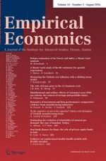
The fit of the Pareto model using the MLE and robust estimators to the Belgian income distribution in 2005 is shown on a log–log plot in Fig. 1.13 In order to stay within our small-sample setting, we apply the estimators to the 40 highest incomes in the data set. The figure confirms the observation of Alfons et al. (2013) that for the data set at hand there is one extreme outlier, which can have a disproportionally high influence on the estimate of a population parameter of interest. The MLE is very seriously affected by the presence of the outlier. All robust estimators perform much better than the MLE with the PITSE having a small edge over the OBRE and the WMLE (the latter two estimators produce almost identical estimates, which are indistinguishable on the figure). The GME does a slightly worse job.
Fig. 1
The empirical complementary cumulative distribution function, P(x), and the fitted various estimators for the Pareto tail index, 40 highest disposable equivalized incomes for Belgium in 2005 (EU-SILC data)
×
Let us assume now that we are interested in the problem of measuring income inequality among the rich persons and that the rich are represented in our sample by the 40 top income observations.14 Since the total sample size for the Belgian data from 2005 is 5,133, the rich defined in our way constitute about 0.8 % of the total sample. The Gini inequality index for our 40 highest income observations, \(\hat{{G}}\), computed nonparametrically, is 0.6481. However, the same index computed excluding the outlying highest income, \(\hat{{G}}_{E}\), is only 0.2468. This shows that the influence of the extreme outlier on statistics computed using tail observations can be indeed very high. Table 15 presents values of the Gini index for the rich implied by the fitted Pareto models with different estimators of the Pareto tail index.15
Table 15
Pareto tail indices estimated using MLE and robust estimators and implied Gini indices, 40 highest disposable equivalized incomes for Belgium in 2005 (EU-SILC data)
Estimator
Pareto tail index
Gini index
MLE
2.0111
0.3309 (0.1093)
OBRE
2.4778
0.2546 (0.0742)
WMLE
2.4818
0.2523 (0.0705)
PITSE
2.5665
0.2420 (0.0683)
GME
2.3782
0.2662 (0.0844)
The estimators are applied to the 40 highest incomes in the data set. The nonparametric Gini index for all observations is 0.6481, excluding the highest income it is 0.2468. Standard errors for the Gini indices implied by the fitted Pareto models appear in parentheses. They were computed using the standard bootstrap with 1000 replications
All parametric estimates of the Gini index give much smaller values than the nonparametric estimate \(\hat{{G}}\), which is destroyed by the presence of the outlier. However, the parametric estimate implied by the MLE (0.3309) is still much higher than the nonparametric estimate computed for the data set excluding the outlier \(\hat{{G}}_{E}\). In general, all parametric estimates of the Gini implied by robust estimators of the tail index are similar and much closer to \(\hat{{G}}_{E}\). However, the PITSE is able to reconstruct the value of the Gini index, which is the closest to \(\hat{{G}}_{E}\), and the variability of the Gini implied by this estimator is comparable or slightly smaller than that of other estimators. This evidence confirms the conclusion from our simulation study that the PITSE should be the preferred choice in applied work using Pareto tail modelling in small samples.
5 Conclusions
The classical Pareto distribution is widely used in many areas of economics and other sciences to model the right tail of heavy-tailed distributions. Since the most popular method of estimating the shape parameter (the Pareto tail index) of this distribution—the maximum likelihood estimation—is non-robust to model deviation and data contamination, several robust approaches have been proposed in the literature. In this paper, we have provided an extensive Monte Carlo comparison of the small-sample performance of the most popular robust estimators for the Pareto tail index.
The main conclusions from our simulation study are the following.16 First, the MLE indeed performs unreliably with even a moderate degree of model deviation or data contamination. Our simulations suggest also that the performance of the MLE deteriorates significantly with the rise in the value of the Pareto tail index. Second, there are computational problems with the PDCE for small samples \((n \le 80)\). The performance of the PDCE is similar to that of other robust estimators only for the largest sample size in our study (200 observations). For these reasons, we recommend that the PDCE should be avoided in practical small-sample settings \((n < 200)\). Third, the WMLE usually performs worse than most of other robust estimators, but shows good results in samples of size 200. Therefore, this estimator should be only used in sufficiently large samples. Fourth, the OBRE, PITSE and GME offer a similar level of protection in most of the studied settings. Taking into account the fact that the PITSE is the simplest estimator from the computational point of view, while both remaining alternatives (and especially the OBRE) are much more complex computationally, the PITSE seems to give the desired compromise between ease of use and power to protect against outliers in the small-sample setting.
Acknowledgments
I would like to thank two anonymous referees for their helpful comments and suggestions. This work was supported by Polish National Science Centre grant no. 2011/01/B/HS4/02809.
Open AccessThis article is distributed under the terms of the Creative Commons Attribution 4.0 International License (http://creativecommons.org/licenses/by/4.0/), which permits unrestricted use, distribution, and reproduction in any medium, provided you give appropriate credit to the original author(s) and the source, provide a link to the Creative Commons license, and indicate if changes were made.
Other non-robust methods of estimation the Pareto tail index, including regression estimators, Bayesian estimators, methods based on moments or order statistics, are discussed in Arnold (1983), Johnson, Kotz, and Balakrishnan (1994, cha. 20), and Kleiber and Kotz (2003, cha. 3). See also Gabaix and Ibragimov (2011) for a recent regression-based estimator, which has a reduced bias in small samples.
Robust methods are used in the context of heavy-tailed distributions not only for the purpose of reducing the bias of the tail index estimate. Another purpose is to measure the impact of the influential observations (see, e.g. Dell’Aquila and Embrechts 2006; Hubert et al. 2013). I would like to thank a referee for pointing this out.
In this paper, we are concerned with mainly with outliers at high quantiles in the right tail of the distribution. Some of the robust estimators of the Pareto tail index are designed to provide protection against departures in the lower quantiles (see, e.g. Beran and Schell 2012). They are not included in our comparison, since this type of outliers is rather unusual.
Since all robust estimators considered in this paper, except the PDCE, allow for the trade-off between efficiency and robustness, the regulating parameters for these estimators were adjusted to match the assumed common levels of ARE. The levels of 78 and 94 % were chosen because the regulating parameter for the GME (see Sect. 2.4) takes only integer values, which restricts the range of admissible values of ARE.
Brazauskas and Serfling (2001b) have also compared their generalized median estimators with some well-established robust and non-robust estimators including method of moments estimators, trimmed mean estimators, regression estimators, least squares estimators, and quantile-based estimators. They concluded that among these estimators the GMEs perform best with respect to the efficiency versus robustness trade-off.
It should be noted here that the estimator of Vandewalle et al. (2007) is designed for Pareto-type distributions defined as \(1-F(x)=x^{-\alpha }l_{F}(x)\), where F(x) is the distribution function and \(l_{F}\) is a slowly varying function. The strict Pareto model (1) holds when \(l_{F}(x)=x_{0}^{\alpha }\). The Pareto-type class includes also Fréchet, Burr, log-gamma and many other distributions (see Beirlant et al. 2004).
For this reason, we do not discuss the performance of the PDCE further in this section. The bad performance of the PDCE in our small-sample setting may be explained by the fact that the estimator was designed for Pareto-type distributions, not only for the strict Pareto model.
Table 1
Simulation results for the Pareto tail index with data drawn from an uncontaminated Pareto distribution \(P(1,\alpha )\), ARE = 94 %
Estimator
\(n = 20\)
\(n = 40\)
\(n = 60\)
\(n = 80\)
\(n = 100\)
\(n = 200\)
RB
RRMSE
RB
RRMSE
RB
RRMSE
RB
RRMSE
RB
RRMSE
RB
RRMSE
\(\alpha = 1\)
MLE
\(-0.2\)
23.8
0.0
16.2
0.0
13.4
\(-0.1\)
11.4
0.2
10.0
\(-0.1\)
7.0
OBRE
9.6
28.8
4.7
18.3
3.0
14.5
2.1
12.3
1.9
10.7
0.8
7.4
PITSE
11.9
30.2
5.8
18.7
3.8
14.8
2.7
12.4
2.4
10.9
1.1
7.5
PDCE
–
–
–
–
51.1
360.9
25.8
117.2
17.8
48.3
7.6
25.2
GME
\(-2.7\)
24.1
\(-0.4\)
16.7
\(-0.3\)
13.8
\(-0.3\)
11.8
0.0
10.3
\(-0.2\)
7.3
\(\alpha = 2\)
MLE
\(-0.2\)
24.2
0.3
16.6
0.0
13.3
\(-0.1\)
11.3
0.1
10.1
\(-0.2\)
7.0
OBRE
9.7
29.4
4.9
18.6
2.9
14.3
2.2
12.2
1.9
10.8
0.6
7.3
PITSE
12.0
30.6
6.0
19.1
3.7
14.7
2.7
12.4
2.4
11.0
0.9
7.3
PDCE
–
–
–
–
35.6
271.7
–
–
14.3
73.1
4.4
18.2
GME
\(-2.6\)
24.4
\(-0.3\)
17.0
\(-0.4\)
13.6
\(-0.2\)
11.7
\(-0.1\)
10.4
\(-0.3\)
7.1
\(\alpha = 3\)
MLE
0.0
24.5
0.1
16.8
0.0
13.3
0.5
11.5
0.3
10.0
0.1
7.2
OBRE
9.8
29.3
4.8
18.9
3.0
14.4
2.6
12.4
2.0
10.6
0.9
7.6
PITSE
12.1
30.7
5.8
19.2
3.7
14.7
3.2
12.5
2.4
10.7
1.1
7.6
PDCE
–
–
–
–
24.6
129.7
14.5
44.1
9.9
28.6
4.1
16.6
GME
\(-2.5\)
24.4
\(-0.4\)
17.3
\(-0.3\)
13.6
0.2
11.8
0.1
10.3
0.0
7.4
RB denotes relative bias, while RRMSE is relative root-mean-square error
Table 2
Simulation results for the Pareto tail index with data drawn from an uncontaminated Pareto distribution \(P(1,\alpha )\), ARE = 78 %
Disposable income is post-tax post-benefit income. Household incomes are equivalized in order to account for differences in the size and age composition of households. The equivalence scale used is the standard EU-SILC scale, which gives a weight of 1 to the first adult household member, then a weight of 0.5 to any subsequent adult and a weight of 0.3 to every child (aged 14+).
We could be interested in estimating inequality among the rich for the purposes of computing an index of richness, which evaluates the overall situation of the rich (see, e.g. Peichl et al. 2010) or for the purposes of computing a semi-parametric inequality index. The latter is a sum of a nonparametric inequality measure estimated for the non-rich and a parametric inequality index for the rich (see, e.g. Cowell and Flachaire 2007).
One limitation of our study is that our simulated data are independent. However, in practice economic and other data are often dependent (e.g. correlated across time or space), which could distort the behaviour of Pareto tail estimators and imply a different ranking of the estimators compared in this paper. I would like to thank a referee for this remark.
 The IF describes the effect of a small contamination \((\varepsilon \delta _{x})\) at a point x on the estimate of \(T_{n}\), standardized by the mass of the contamination. Linear approximation \(\varepsilon ~\hbox {IF}(x; T; F_{\theta })\) measures therefore the asymptotic bias of the estimator caused by the contamination. In case of the MLE, the IF is proportional to the score function \(s(x;\theta )=\frac{\partial }{\partial \theta }\log f_\theta (x)\), which for the Pareto distribution is \(s(x;\alpha )=1/\alpha -\log x+\log x_{0}\). Since this function is unbounded in x, the MLE for \(\alpha \) is not robust. A robust estimator possessing a bounded IF is called B-robust (or biased-robust).