Top
Published in: Neural Computing and Applications 1/2022

Open Access 24-11-2020 | S.I. : WSOM 2019

Quantum-inspired learning vector quantizers for prototype-based classification

Confidential: for personal use only—submitted to Neural Networks and Applications 5/2020

Authors: Thomas Villmann, Alexander Engelsberger, Jensun Ravichandran, Andrea Villmann, Marika Kaden

Published in: Neural Computing and Applications | Issue 1/2022

Activate our intelligent search to find suitable subject content or patents.

search-config
loading …

Abstract

Prototype-based models like the Generalized Learning Vector Quantization (GLVQ) belong to the class of interpretable classifiers. Moreover, quantum-inspired methods get more and more into focus in machine learning due to its potential efficient computing. Further, its interesting mathematical perspectives offer new ideas for alternative learning scenarios. This paper proposes a quantum computing-inspired variant of the prototype-based GLVQ for classification learning. We start considering kernelized GLVQ with real- and complex-valued kernels and their respective feature mapping. Thereafter, we explain how quantum space ideas could be integrated into a GLVQ using quantum bit vector space in the quantum state space \({\mathcal {H}}^{n}\) and show the relations to kernelized GLVQ. In particular, we explain the related feature mapping of data into the quantum state space \({\mathcal {H}}^{n}\). A key feature for this approach is that \({\mathcal {H}}^{n}\) is an Hilbert space with particular inner product properties, which finally restrict the prototype adaptations to be unitary transformations. The resulting approach is denoted as Qu-GLVQ. We provide the mathematical framework and give exemplary numerical results.
Notes

Publisher's Note

Springer Nature remains neutral with regard to jurisdictional claims in published maps and institutional affiliations.

1 Introduction

Classification learning still belongs to the main tasks in machine learning [5]. Although powerful methods are available, still there is need for improvements and search for alternatives to the existing strategies. A huge progress was achieved by the realization of deep networks [15, 28]. These networks overcame the hitherto dominating support vector machines (SVM) in classification learning [11, 51]. However, deep architectures have the disadvantage that the interpretability is at least difficult. Therefore, great effort is currently spent to explain deep models, see [40] and references therein. However, due to the complexity of deep networks this is quite often impossible [70]. Thus, alternatives are required for many applications like in medicine [39]. A promising alternative is the concept of distance-based methods like in learning vector quantizations [57], where prototypes play the role to be references for data [25, 34, 37]. Further, prototype layers in deep networks also seem to stabilize the behavior deep models [29].
Learning vector quantizers (LVQ) are sparse models for prototype-based classification learning, which were heuristically introduced by T. Kohonen [23, 24]. LVQ is a competitive learning algorithm relying on an attraction and repulsion scheme (ARS) for prototype adaptation, which can be described geometrically in case of the Euclidean setting. Keeping the idea of ARS but take the LVQ to the next level is the generalized LVQ (GLVQ), which optimizes a loss function approximating the classification error [42]. Standard training is stochastic gradient descent learning (SGDL) based on the local losses.
Of particular interest for potential users is the advantage of easy interpretability of LVQ networks according to the prototype principle [63]. Further, LVQ networks belong to the class of classification margin optimizers like SVM [10] and are proven to be robust against adversarial attacks [41].
In standard LVQ networks, the distance measure is set to be the squared Euclidean one, yet other proximities can be applied [4]. For example, in case of spectral data or histograms, divergences are beneficial [21, 31, 58], whereas functional data may benefit from similarities including aspects of the slope like Sobolev distances [60]. Even the kernel trick successfully applied in SVM can be adopted to the GLVQ, denoted as kernelized GLVQ (KGLVQ [59], i.e., the data and prototypes are implicitly mapped into a potentially infinite-dimensional Hilbert space but compared by means of the kernel-based distance calculated in the low-dimensional data space [45]. For reproducing kernel Hilbert spaces, the respective mapping is unique [52, 53]. This so-called feature mapping frequently is nonlinear depending on the kernel in use [17].
However, SGDL training for KGLVQ requires differentiability of the kernel. Otherwise, median variants of GLVQ have to be considered, i.e., the prototype is restricted to be data points and the optimization goes back to likelihood optimization [32]. Replacing the standard Euclidean distance by nonlinear kernel distances can improve the performance of the GLVQ model as it is known for the SVM. Yet, the maybe improved performance of KGLVQ comes with a weaker interpretability, because the implicit kernel mapping does not allow to observe the mapped data directly in the feature space.
Another way to accelerate the usually time-consuming training process in machine learning models is to make use of efficient quantum computing algorithms [9, 12, 33]. For supervised and unsupervised problems, several approaches are developed [3, 46, 49, 50, 64]. A recent overview for recently developed quantum-inspired approaches can be found in [26].
Quantum support vector machines are studied in [36], Hopfield networks are investigated in [35]. A quantum perceptron algorithm is proposed in [66]. Particularly, nearest neighbor approaches are studied in [19, 65]. Related to vector quantization, the c-means algorithm is considered in [22, 69], which can be also seen in connection to quantum classification algorithms based on competitive learning [71].
In this contribution, we propose an alternative nonlinear data processing but somewhat related to kernel GLVQ keeping the idea to map the data nonlinearly into a particular Hilbert space. In particular, we transform the data vectors nonlinearly into quantum state vectors and require at the same time that the prototypes are always quantum state vectors, too [48, 61]. The respective quantum space also is a Hilbert space, and hence, we can take the data mapping as some kind of feature mapping like for kernels [16, 56]. The adaptation has to ensure the attraction and repulsing strategy known to be the essential ingredients of LVQ algorithms, but has to be adapted here to quantum state space properties. The latter restriction requires the adaptations to be unitary transformations. The resulting algorithm is denoted as Quantum-inspired GLVQ (Qu-GLVQ).
In fact, quantum-inspired machine learning algorithms seem to be a promising approach to improve effectiveness of algorithms with respect to time complexity [55]. Yet, here the benefit would be twice because we also emphasize the mathematical similarity to kernel-based learning, which still is one of the most successful strategies in machine learning [53, 59]. However, a realization on a real quantum system is not in the focus of this paper and, hence, left for future work. The focus of this paper is clearly to show the mathematical similarities between kernel and quantum approaches.
The paper is structured as follows: Starting with a short introduction of standard GLVQ for real and complex data [14], we briefly explain the use of real and complex kernels in context of GLVQ. Again, we consider both the real and the complex case. After these preliminaries, we give the basic mathematical properties of quantum state spaces and incorporating these concepts into GLVQ. We show that this approach is mathematically consistent with the kernel GLVQ. Numerical simulations exemplary show the successful application of the introduced Qu-GLVQ.
Further, we emphasize that the aim of the paper is not to show any improvement in quantum-inspired GLVQ compared to kernel approaches or standard GLVQ. Instead, one goal is to show that both the quantum and the kernel approach are mathematically more or less equivalent while kernel approaches apply implicit mapping and the quantum approach does the mapping explicitly.

2 The general GLVQ approach

2.1 GLVQ for real valued data

Standard GLVQ as introduced in [42] assumes data vectors \(\mathbf {v}\in V\subseteq \mathbb {R}^{n}\) with class labels \(c\left( \mathbf {v}\right) \in \mathcal {C}=\left\{ 1,\ldots ,C\right\} \) for training. It is a cost function-based variant of standard LVQ as introduced by T. Kohonen [23, 24] keeping the ARS. Further, a set \(P=\left\{ \mathbf {p}_{k}\right\} _{k=1}^{K}\subset \mathbb {R}^{n}\) of prototypes with class labels \(c_{k}=c\left( \mathbf {p}_{k}\right) \) is supposed together with a differentiable dissimilarity measure \(d\left( \mathbf {v},\mathbf {p}_{k}\right) \) frequently chosen as the (squared) Euclidean distance. Classification of an unknown data sample takes place as a nearest prototype decision with the class label of the winning prototype as response. GLVQ considers the cost function
$$\begin{aligned} E_{GLVQ}\left( V,P\right) =\sum _{\mathbf {v}\in V}L\left( \mathbf {v},P\right) \end{aligned}$$
for optimization of the prototypes. Here
$$\begin{aligned} L\left( \mathbf {v},P\right) =f\left( \mu \left( \mathbf {v}\right) \right) \end{aligned}$$
(1)
is the local loss and f is the transfer function frequently chosen as sigmoid. The classifier function
$$\begin{aligned} \mu \left( \mathbf {v}\right) =\frac{d^{+}\left( \mathbf {v}\right) -d^{-}\left( \mathbf {v}\right) }{d^{+}\left( \mathbf {v}\right) +d^{-}\left( \mathbf {v}\right) } \end{aligned}$$
(2)
takes value in the interval \(\left[ -1,1\right] \), where \(d^{\pm }\left( \mathbf {v}\right) =d\left( \mathbf {v},\mathbf {p}^{\pm }\right) \) is the dissimilarity of a given input to the best matching correct/incorrect prototype \(\mathbf {p}^{\pm }\) regarding the class labels. The classifier function \(\mu \left( \mathbf {v}\right) \) delivers negative values for correct classification. Thus, \(E_{GLVQ}\left( V,P\right) \) approximates the classification error an is optimized by stochastic gradient descent learning (SGDL, [38]) regarding the prototypes according to
$$\begin{aligned} \varDelta \mathbf {p}^{\pm }\propto -\frac{\partial L\left( \mathbf {v},P\right) }{\partial \mathbf {p}^{\pm }}=-\frac{\partial f\left( \mu \left( \mathbf {v}\right) \right) }{\partial \mu }\frac{\partial \mu \left( \mathbf {v}\right) }{\partial d^{\pm }}\frac{\partial d^{\pm }\left( \mathbf {v}\right) }{\partial \mathbf {p}^{\pm }} \end{aligned}$$
(3)
as local derivatives. In fact, this learning rule realizes the ARS in case of the squared Euclidean distance, because of \(\frac{\partial d^{\pm }\left( \mathbf {v}\right) }{\partial \mathbf {p}^{\pm }}=-2\left( \mathbf {v}-\mathbf {p}^{\pm }\right) \). As mentioned before, this standard GLVQ constitutes a margin classifier and is robust against adversarial attacks [10, 41].
If the expression
$$\begin{aligned} d_{\varvec{\varOmega }}\left( \mathbf {v},\mathbf {p}\right) =\left( \varvec{\varOmega }\left( \mathbf {v}-\mathbf {p}\right) \right) ^{2} \end{aligned}$$
(4)
describes a standard quadratic form with \(\varvec{\varOmega }\in \mathbb {R}^{m\times n}\), we can calculate the derivative accordingly by
$$\begin{aligned} \frac{\partial d_{\varvec{\varOmega }}\left( \mathbf {v},\mathbf {p}\right) }{\partial \mathbf {p}}=-2\varvec{\varOmega }^{T}\varvec{\varOmega }\left( \mathbf {v}-\mathbf {p}\right) \end{aligned}$$
(5)
whereas
$$\begin{aligned} \frac{\partial d_{\varvec{\varOmega }}\left( \mathbf {v},\mathbf {p}\right) }{\partial \varvec{\varOmega }}=\varvec{\varOmega }\left( \mathbf {v}-\mathbf {p}\right) \left( \mathbf {v}-\mathbf {p}\right) ^{T} \end{aligned}$$
(6)
yields an adaptation \(\varDelta \varvec{\varOmega }\) of the matrix \(\varvec{\varOmega }\) [8, 43]. The adaptation of the \(\varvec{\varOmega }\)-matrix realizes an classification task-specific metric adaptation for optimum class separation [44]. This matrix learning variant of GLVQ is denoted as GMLVQ.
For the (real-valued) kernel GLVQ (KGLVQ) discussed in [59], the dissimilarity measure \(d\left( \mathbf {v},\mathbf {p}\right) \) is set to be the (squared) kernel distance
$$\begin{aligned} d_{\kappa }\left( \mathbf {v},\mathbf {p}\right) =\kappa \left( \mathbf {v},\mathbf {v}\right) -2\kappa \left( \mathbf {v},\mathbf {p}\right) +\kappa \left( \mathbf {p},\mathbf {p}\right) \end{aligned}$$
(7)
with the differentiable kernel \(\kappa \) and the respective (implicit) real kernel feature mapping \(\varPhi _{\kappa }:\mathbb {R}^{n}\rightarrow H\) into the (real) reproducing kernel Hilbert space H [53]. As mentioned in the introduction, the implicitly mapped data \(\varPhi _{\kappa }\left( \mathbf {v}\right) \) form a low-dimensional manifold \(D_{\varPhi }\left( V\right) \) in the feature mapping space H whereas the prototypes \(\varPhi _{\kappa }\left( \mathbf {p}\right) \) are allowed to move freely in H and, hence may leave \(D_{\varPhi }\left( V\right) \). In this case, the prototypes recognize the data from outside, which could be a disadvantage for particular applications.

2.2 Complex variants of GLVQ

So far we assumed both \(\mathbf {v}\in V\subseteq \mathbb {R}^{n}\) and \(P=\left\{ \mathbf {p}_{k}\right\} \subset \mathbb {R}^{n}\) for data and prototypes as well as \(\varvec{\varOmega }\in \mathbb {R}^{m\times n}\). In complex GLVQ, all these quantities are assumed to be complex valued. The squared distance (4) reads as
$$\begin{aligned} d_{\varvec{\varOmega }}\left( \mathbf {v},\mathbf {p}\right) =\left( \mathbf {v}-\mathbf {p}\right) ^{*}\varvec{\varOmega }^{*}\varvec{\varOmega }\left( \mathbf {v}-\mathbf {p}\right) \end{aligned}$$
where \(\left( \mathbf {v}-\mathbf {p}\right) ^{*}\varvec{\varOmega }^{*}=\left( \varvec{\varOmega }\left( \mathbf {v}-\mathbf {p}\right) \right) ^{*}\) is the Hermitian conjugate of \(\varvec{\varOmega }\left( \mathbf {v}-\mathbf {p}\right) \). Following [14, 54], the derivatives according to (5) and (6) are obtained by the Wirtinger calculus (see “Appendix 6”) applying the conjugate derivatives as
$$\begin{aligned} \frac{\partial _{\mathfrak {W}}d_{\varvec{\varOmega }}\left( \mathbf {v},\mathbf {p}\right) }{\partial \mathbf {p}^{*}}=-2\varvec{\varOmega }^{*}\varvec{\varOmega }\left( \mathbf {v}-\mathbf {p}\right) \end{aligned}$$
(8)
whereas
$$\begin{aligned} \frac{\partial _{\mathfrak {W}}d_{\varvec{\varOmega }}\left( \mathbf {v},\mathbf {p}\right) }{\partial \varvec{\varOmega }^{*}}=\varvec{\varOmega }\left( \mathbf {v}-\mathbf {p}\right) \left( \mathbf {v}-\mathbf {p}\right) ^{*} \end{aligned}$$
(9)
,respectively, which have to be plugged into (3).
For complex kernels \(\kappa :\mathbb {C}^{n}\times \mathbb {C}^{n}\rightarrow \mathbb {C}\) we get
$$\begin{aligned} d_{\kappa }\left( \mathbf {v},\mathbf {p}\right) =\kappa \left( \mathbf {v},\mathbf {v}\right) -2\mathfrak {Re}\left( \kappa \left( \mathbf {v},\mathbf {p}\right) \right) +\kappa \left( \mathbf {p},\mathbf {p}\right) \end{aligned}$$
(10)
instead of (7) using the identity \({{\mathfrak {Re}\left( \kappa \left( \mathbf {v},\mathbf {p}\right) \right) }=}\kappa \left( \mathbf {v},\mathbf {p}\right) +\kappa \left( \mathbf {p},\mathbf {v}\right) \). Provided that the kernel \(\kappa \) is differentiable in the sense of Wirtinger [6, 7], the derivative of the kernel distance becomes
$$\begin{aligned} \frac{\partial _{\mathfrak {W}}d_{\kappa }\left( \mathbf {v},\mathbf {p}\right) }{\partial \mathbf {p}^{*}}= & {} -2\frac{\partial _{\mathfrak {W}}\mathfrak {Re}\left( \kappa \left( \mathbf {v},\mathbf {p}\right) \right) }{\partial \mathbf {p}^{*}}\\ \\= & {} -\frac{\partial _{\mathfrak {W}}\kappa \left( \mathbf {v},\mathbf {p}\right) }{\partial \mathbf {p}^{*}}-\frac{\partial _{\mathfrak {W}}\kappa \left( \mathbf {p},\mathbf {v}\right) }{\partial \mathbf {p}^{*}} \end{aligned}$$
paying attention to \(\frac{\partial _{\mathfrak {W}}\kappa \left( \mathbf {v},\mathbf {v}\right) }{\partial \mathbf {p}^{*}}=\frac{\partial _{\mathfrak {W}}\kappa \left( \mathbf {p},\mathbf {p}\right) }{\partial \mathbf {p}^{*}}=0\). This derivative has to be taken into account to calculate the prototype update (3).

3 Quantum-inspired GLVQ

In the following we explain our idea of a quantum-inspired GLVQ. For this purpose, first we briefly introduce quantum state vectors and consider their transformations. Subsequently, we describe the proposed network architecture for both the real and the complex case. Finally, we explain, how to map real or complex data into a quantum state space by application of nonlinear mappings. This nonlinear mappings play the role of kernel feature maps as known from kernel methods.

3.1 Quantum bits, quantum state vectors and transformations

3.1.1 The real case

Quantum-inspired machine learning gains more and more attention [9, 33, 49]. Following the usual notations, the data are required to be quantum bits (qubits)
$$\begin{aligned} \left| x\right\rangle= \alpha \left( \left| x\right\rangle \right) \cdot \left| 0\right\rangle +\beta \left( \left| x\right\rangle \right) \cdot \left| 1\right\rangle \end{aligned}$$
(11)
$$\begin{aligned}= \left[ \begin{array}{c} \alpha \left( \left| x\right\rangle \right) \\ \beta \left( \left| x\right\rangle \right) \end{array}\right] \end{aligned}$$
(12)
with the normalization condition
$$\begin{aligned} \left| \alpha \left( \left| x\right\rangle \right) \right| ^{2}+\left| \beta \left( \left| x\right\rangle \right) \right| ^{2}=1 \end{aligned}$$
(13)
defining the Bloch-sphere [68]. In this real case, we suppose both \(\alpha \left( \left| x\right\rangle \right) ,\beta \left( \left| x\right\rangle \right) \in \mathbb {R}\).1 The normalization condition is equivalent to
$$\begin{aligned} \alpha \left( \left| x\right\rangle \right) =\cos \left( \xi \right) \text { and }\beta \left( \left| x\right\rangle \right) =\sin \left( \xi \right) \end{aligned}$$
(14)
for an angle \(\xi \in \left[ 0,2\pi \right] \) paying attention to the periodicity of the cosinus function.
Consequently, we get the inner product for the quantum states \(\left| x\right\rangle \) and \(\left| w\right\rangle \) as
$$\begin{aligned} \left\langle x|w\right\rangle =\alpha \left( \left| x\right\rangle \right) \alpha \left( \left| w\right\rangle \right) +\beta \left( \left| x\right\rangle \right) \beta \left( \left| w\right\rangle \right) \end{aligned}$$
(15)
as the Euclidean inner product of the amplitude vectors \(\left[ \begin{array}{c} \alpha \left( \left| x\right\rangle \right) \\ \beta \left( \left| x\right\rangle \right) \end{array}\right] = \left[ \begin{array}{c} \cos \left( \xi \right) \\ \sin \left( \xi \right) \end{array}\right]\) and \(\left[ \begin{array}{c} \alpha \left( \left| w\right\rangle \right) \\ \beta \left( \left| w\right\rangle \right) \end{array}\right] =\left[ \begin{array}{c} \cos \left( \omega \right) \\ \sin \left( \omega \right) \end{array}\right] \). Hence, we have \(\left\langle x|x\right\rangle =1\) such that the (squared) qubit distance \(\delta \) can be calculated as
$$\begin{aligned} \delta \left( \left| x\right\rangle ,\left| w\right\rangle \right) =2\cdot \left( 1-\left\langle x|w\right\rangle \right) \,. \end{aligned}$$
(16)
Transformations \(\mathbf {U}\left[ \begin{array}{c} \alpha \left( \left| x\right\rangle \right) \\ \beta \left( \left| x\right\rangle \right) \end{array}\right] =\mathbf {U}\left| x\right\rangle \) of qubits are realized by orthonormal matrices \(\mathbf {U}\in \mathbb {R}^{2\times 2}\), i.e., \(\mathbf {U}\cdot \mathbf {U}^{T}=\mathbf {E}\) with \(\mathbf {U}^{T}\) is the transpose. Note that the application of orthonormal matrices remains the inner product invariant, i.e., \(\left\langle \mathbf {U}x|\mathbf {U}y\right\rangle =\left\langle x|y\right\rangle \) and form the orthonormal group with matrix multiplication as group operation [13].
Now, we define qubit data vectors as \(\left| \mathbf {x}\right\rangle =\left( \left| x_{1}\right\rangle ,\ldots ,\left| x_{n}\right\rangle \right) ^{T}\) with qubits \(\left| x_{k}\right\rangle \) and the vector \(\left| \mathbf {w}\right\rangle =\left( \left| w_{1}\right\rangle ,\ldots ,\left| w_{n}\right\rangle \right) ^{T}\) for prototypes. For the inner product, we get \(\left\langle \mathbf {x}|\mathbf {w}\right\rangle _{\mathcal {H}^{n}}=\sum _{k=1}^{n}\left\langle x_{k}|w_{k}\right\rangle \) with
$$\begin{aligned} \left| w_{k}\right\rangle =\cos \left( \omega _{k}\right) \cdot \left| 0\right\rangle +\sin \left( \omega _{k}\right) \cdot \left| 1\right\rangle \end{aligned}$$
and \(\left\langle \mathbf {x}|\mathbf {x}\right\rangle =\left\langle \mathbf {w}|\mathbf {w}\right\rangle =n\). Thus, we get
$$\begin{aligned} \delta \left( \left| \mathbf {x}\right\rangle ,\left| \mathbf {w}\right\rangle \right) =2\left( n-\left\langle \mathbf {x}|\mathbf {w}\right\rangle _{\mathcal {H}^{n}}\right) \end{aligned}$$
(17)
as the squared distance between qubit vectors. Using (15), we obtain
$$\begin{aligned} \delta \left( \left| \mathbf {x}\right\rangle ,\left| \mathbf {w}\right\rangle \right) =2\left( n-\sum _{k=1}^{n}\cos \left( \xi _{k}\right) \cos \left( \omega _{k}\right) +\sin \left( \xi _{k}\right) \sin \left( \omega _{k}\right) \right) \end{aligned}$$
(18)
in terms of the amplitude values.
Orthogonal transformations of qubit vectors are realized by block-diagonal matrices according to \(\mathbf {U}^{\left( n\right) }\left| \mathbf {x}\right\rangle =\text {diag}\left( \mathbf {U}_{1},\ldots ,\mathbf {U}_{n}\right) \cdot \left| \mathbf {x}\right\rangle \). Obviously, the quantum space \(\mathcal {H}^{n}\) of n-dimensional qubit vectors is an Hilbert space with the inner product \(\left\langle \mathbf {x}|\mathbf {w}\right\rangle _{\mathcal {H}^{n}}\) as also recognized in [46, 48].

3.1.2 The complex case

In the complex-valued case, the data are required to be quantum bits (qubits), too but now taken as
$$\begin{aligned} \left| x\right\rangle= \alpha \left( \left| x\right\rangle \right) \cdot \left| 0\right\rangle +\beta \left( \left| x\right\rangle \right) \cdot e^{i\phi }\cdot \left| 1\right\rangle \end{aligned}$$
(19)
$$\begin{aligned}= \left[ \begin{array}{c} \alpha \left( \left| x\right\rangle \right) \\ \beta \left( \left| x\right\rangle \right) \cdot e^{i\phi } \end{array}\right] \end{aligned}$$
(20)
with coefficients \(\alpha \left( \left| x\right\rangle \right) ,\beta \left( \left| x\right\rangle \right) \in \mathbb {R}\) and the complex phase information \(e^{i\phi }\). The normalization condition for the Bloch sphere becomes
$$\begin{aligned} 1= & {} \,\left| \alpha \left( \left| x\right\rangle \right) \right| ^{2}+\left| \beta \left( \left| x\right\rangle \right) \cdot e^{i\phi }\right| ^{2}\nonumber \\ \nonumber \\= & {} \,\left| \alpha \left( \left| x\right\rangle \right) \right| ^{2}+\left| \beta \left( \left| x\right\rangle \right) \right| ^{2}\cdot \underset{=1}{\underbrace{\left| e^{i\phi }\right| ^{2}}} \end{aligned}$$
(21)
and, hence, the amplitudes are again as in (14). The complex-valued inner product \(\left\langle x|w\right\rangle \) for \(\left| w_{l}\right\rangle =\cos \left( \omega _{l}\right) \cdot \left| 0\right\rangle +\sin \left( \omega _{l}\right) \cdot e^{i\psi }\cdot \left| 1\right\rangle \) is calculated as
$$\begin{aligned} \left\langle x|w\right\rangle= & {} \alpha \left( \left| x\right\rangle \right) \cdot \overline{\alpha \left( \left| w\right\rangle \right) }+\beta \left( \left| x\right\rangle \right) \cdot e^{i\phi }\cdot \overline{\beta \left( \left| w\right\rangle \right) \cdot e^{i\psi }}\nonumber \\ \nonumber \\= & {} \cos \left( \xi \right) \cos \left( \omega \right) +\sin \left( \xi \right) \sin \left( \omega \right) \cdot e^{i\left( \phi -\psi \right) }\nonumber \\ \nonumber \\= & {} \cos \left( \xi \right) \cos \left( \omega \right) +\sin \left( \xi \right) \sin \left( \omega \right) \cdot \left( \cos \left( \phi -\psi \right) \right. \nonumber \\&\left. +\,i\cdot \sin \left( \phi -\psi \right) \right) \end{aligned}$$
(22)
now depending on both phase information \(\psi \) and \(\phi \). Accordingly, the qubit distance \(\delta \left( \left| x\right\rangle ,\left| w\right\rangle \right) \) is calculated as
$$\begin{aligned} \delta \left( \left| x\right\rangle ,\left| w\right\rangle \right)= & {} \sqrt{\left\langle x|x\right\rangle -\left\langle x|w\right\rangle -\left\langle w|x\right\rangle +\left\langle w|w\right\rangle }\nonumber \\ \nonumber \\= & {} \sqrt{2-\left\langle x|w\right\rangle -\overline{\left\langle x|w\right\rangle }}\nonumber \\ \nonumber \\= & {} \sqrt{2}\cdot \sqrt{1-\mathfrak {Re}\left( \left\langle x|w\right\rangle \right) } \end{aligned}$$
(23)
paying attention to the properties of the complex inner product. Particularly, we have
$$\begin{aligned} \mathfrak {Re}\left( \left\langle x|y\right\rangle \right) =\cos \left( \xi \right) \cos \left( \omega \right) +\sin \left( \xi \right) \sin \left( \omega \right) \cdot \cos \left( \phi -\psi \right) \end{aligned}$$
(24)
for the real part of \(\left\langle x|y\right\rangle \).
Transformations \(\mathbf {U}\left[ \begin{array}{c} \alpha \left( \left| x\right\rangle \right) \\ \beta \left( \left| x\right\rangle \right) \end{array}\right] =\mathbf {U}\left| x\right\rangle \) of complex qubits are realized by unitary matrices \(\mathbf {U}\in \mathbb {C}^{2\times 2}\), i.e., \(\mathbf {U}\cdot \mathbf {U}^{*}=\mathbf {E}\) with \(\mathbf {U}^{*}\) is the Hermitian transpose, where unitary matrices remain the inner product invariant, i.e., \(\left\langle \mathbf {U}x|\mathbf {U}y\right\rangle =\left\langle x|y\right\rangle \). As for orthonormal matrices, the unitary matrices form a group with matrix multiplication as group operation [13].
Using again the normalization condition (13), we obtain
$$\begin{aligned} \delta \left( \left| \mathbf {x}\right\rangle ,\left| \mathbf {w}\right\rangle \right) =2\left( n-\mathfrak {Re}\left( \left\langle \mathbf {x}|\mathbf {w}\right\rangle _{\mathcal {H}^{n}}\right) \right) \end{aligned}$$
(25)
as the squared quantum distance between the qubit vectors. This can be calculated as
$$\begin{aligned}&\delta \left( \left| \mathbf {x}\right\rangle ,\left| \mathbf {w}\right\rangle \right) =2\left( n-\sum _{k=1}^{n}\cos \left( \xi _{k}\right) \cos \left( \omega _{k}\right) \right. \nonumber \\&\quad \left. +\sin \left( \xi _{k}\right) \sin \left( \omega _{k}\right) \cdot \cos \left( \phi _{k}-\psi _{k}\right) \right) \end{aligned}$$
(26)
using (24).
Analogously to the real case, unitary transformations of qubit vectors are realized by block-diagonal matrices according to \(\mathbf {U}^{\left( n\right) }\left| \mathbf {x}\right\rangle =\text {diag}\left( \mathbf {U}_{1},\ldots ,\mathbf {U}_{n}\right) \cdot \left| \mathbf {x}\right\rangle \) and the quantum space \(\mathcal {H}^{n}\) of n-dimensional complex qubit vectors is an Hilbert space with the inner product \(\left\langle \mathbf {x}|\mathbf {w}\right\rangle _{\mathcal {H}^{n}}\).

3.2 The quantum-inspired GLVQ algorithm

3.2.1 The real case

For the real case, we assume a vanishing complex phase information [30], i.e., we require \(\phi =0\) yielding \(e^{i\phi }=1\). Thus, the Qu-GLVQ approach takes real-valued qubit vectors \(\left| \mathbf {x}\right\rangle \) and \(\left| \mathbf {w}\right\rangle \) as elements of the data and the prototype sets X and W, respectively. Hence, the complex phase information yields \(e^{i\phi }=1\) assuming \(\phi =0\) [30]. Thus, the dissimilarity measure \(d^{\pm }\left( \mathbf {v}\right) =d\left( \mathbf {v},\mathbf {p}^{\pm }\right) \) in (2) for GLVQ has to be replaced by the squared qubit vector distance \(\delta \left( \left| \mathbf {x}\right\rangle ,\left| \mathbf {w}\right\rangle \right) \) from (17). All angles \(\omega _{l}\) from \(\left| \mathbf {w}\right\rangle \) form the angle vector \(\varvec{\omega }=\left( \omega _{1},\ldots ,\omega _{n}\right) ^{T}\). The prototype update can be realized adapting the angle vectors in complete analogy to (3) according to
$$\begin{aligned} \varDelta \varvec{\omega }^{\pm }\propto -\frac{\partial L\left( \left| \mathbf {x}\right\rangle ,W\right) }{\partial \varvec{\omega }^{\pm }}=-\frac{\partial f\left( \mu \left( \left| \mathbf {x}\right\rangle \right) \right) }{\partial \mu }\frac{\partial \mu \left( \left| \mathbf {x}\right\rangle \right) }{\partial \delta ^{\pm }}\frac{\partial \delta ^{\pm }\left( \left| \mathbf {x}\right\rangle \right) }{\partial \left| \mathbf {w}\right\rangle } \end{aligned}$$
(27)
where
$$\begin{aligned} \delta ^{\pm }\left( \left| \mathbf {x}\right\rangle \right) =\delta \left( \left| \mathbf {x}\right\rangle ,\left| \mathbf {w}^{\pm }\right\rangle \right) \end{aligned}$$
(28)
is the squared distance to the best matching correct and incorrect prototype. Using the relation (18), we easily obtain
$$\begin{aligned} \frac{\partial \delta ^{\pm }\left( \left| \mathbf {x}\right\rangle \right) }{\partial \omega _{k}^{\pm }}=-\cos \left( \xi _{k}\right) \cdot \sin \left( \omega _{k}^{\pm }\right) +\sin \left( \xi _{k}\right) \cdot \cos \left( \omega _{k}^{\pm }\right) \end{aligned}$$
(29)
delivering the gradient vector \(\frac{\partial \delta ^{\pm }\left( \left| \mathbf {x}\right\rangle \right) }{\partial \varvec{\omega }^{\pm }}\) where
$$\begin{aligned} \frac{\partial \delta ^{\pm }\left( \left| \mathbf {x}\right\rangle \right) }{\partial \omega _{k}^{\pm }}=\frac{\partial \delta ^{\pm }\left( \left| \mathbf {x}\right\rangle \right) }{\partial \left| \mathbf {w}^{\pm }\right\rangle }\frac{\partial \left| \mathbf {w}^{\pm }\right\rangle }{\partial \varvec{\omega }^{\pm }} \end{aligned}$$
(30)
is used. We further remark that (27) together with (29) ensures the prototypes to remain quantum state vectors. Thus, this update corresponds to an orthogonal (unitary) transformations \(\mathbf {U}_{k}\left( \varDelta \omega _{k}\right) \cdot \left| w_{k}\right\rangle \) realizing the update \(\varDelta \left| \mathbf {w}^{\pm }\right\rangle \) directly in the quantum space \(\mathcal {H}^{n}\). Further, we can collect all transformations by \(\mathbf {U}_{k}^{\varSigma }=\varPi _{t=1}^{N}\mathbf {U}_{k}\left( \varDelta \omega _{k}\left( t\right) \right) \) where \(\varDelta \omega _{k}\left( t\right) \) is angle change at time step t. Due to the group property of orthogonal transformations the matrix \(\mathbf {U}_{k}^{\varSigma }\) is also orthogonal and allows to re-calculate the initial state \(\left| w_{k}\right\rangle \) from the final.

3.2.2 The complex case

The complex variant of Qu-GLVQ depends on both \(\varvec{\omega }^{\pm }\) and \(\varvec{\psi }^{\pm }\) according to (26) and, therefore, the angle vector update (27) for \(\varvec{\omega }^{\pm }\) is accompanied by the respective update
$$\begin{aligned} \varDelta \varvec{\psi }^{\pm }\propto -\frac{\partial L\left( \left| \mathbf {x}\right\rangle ,W\right) }{\partial \varvec{\psi }^{\pm }}=-\frac{\partial f\left( \mu \left( \left| \mathbf {x}\right\rangle \right) \right) }{\partial \mu }\frac{\partial \mu \left( \left| \mathbf {x}\right\rangle \right) }{\partial \delta ^{\pm }}\frac{\partial \delta ^{\pm }\left( \left| \mathbf {x}\right\rangle \right) }{\partial \varvec{\psi }^{\pm }}\,, \end{aligned}$$
(31)
for the phase vectors. Again we used the convention
$$\begin{aligned} \frac{\partial \delta ^{\pm }\left( \left| \mathbf {x}\right\rangle \right) }{\partial \varvec{\psi }^{\pm }}=\frac{\partial \delta _{\mathfrak {W}}^{\pm }\left( \left| \mathbf {x}\right\rangle \right) }{\partial \left| \mathbf {w}^{\pm }\right\rangle }\frac{\partial \left| \mathbf {w}^{\pm }\right\rangle }{\partial \varvec{\psi }^{\pm }} \end{aligned}$$
similar as before but taking the Wirtinger derivative, see “Appendix 6”. However, we can avoid the explicit application of the Wirtinger calculus: Using (24), we obtain now for (30)
$$\begin{aligned} \frac{\partial \delta ^{\pm }\left( \left| \mathbf {x}\right\rangle \right) }{\partial \omega _{k}^{\pm }}= & {} \frac{\partial \delta ^{\pm }\left( \left| \mathbf {x}\right\rangle \right) }{\partial \omega _{k}^{\pm }}\left( \cos \left( \xi _{k}\right) \cdot \cos \left( \omega _{k}^{\pm }\right) \right. \\&\left. +\sin \left( \xi _{k}\right) \cdot \sin \left( \omega _{k}^{\pm }\right) \cdot \cos \left( \phi _{k}-\psi _{k}^{\pm }\right) \right) \\ \\= & {} -\cos \left( \xi _{k}\right) \cdot \sin \left( \omega _{k}^{\pm }\right) \\&+\sin \left( \xi _{k}\right) \cdot \cos \left( \omega _{k}^{\pm }\right) \cdot \cos \left( \phi _{k}-\psi _{k}^{\pm }\right) \end{aligned}$$
determining \(\varDelta \varvec{\omega }^{\pm }\) via (27) and again avoiding the explicit application of the Wirtinger calculus. Further, we get
$$\begin{aligned} \frac{\partial \delta ^{\pm }\left( \left| \mathbf {x}\right\rangle \right) }{\partial \psi _{k}^{\pm }}= & {} \frac{\partial \delta ^{\pm }\left( \left| \mathbf {x}\right\rangle \right) }{\partial \psi _{k}^{\pm }}\left( \cos \left( \xi _{k}\right) \cdot \cos \left( \omega _{k}^{\pm }\right) \right. \\&\left. +\sin \left( \xi _{k}\right) \cdot \sin \left( \omega _{k}^{\pm }\right) \cdot \cos \left( \phi _{k}-\psi _{k}^{\pm }\right) \right) \\= & {} \cos \left( \xi _{k}\right) \cdot \cos \left( \omega _{k}^{\pm }\right) \\&+\sin \left( \xi _{k}\right) \cdot \sin \left( \omega _{k}^{\pm }\right) \cdot \sin \left( \phi _{k}-\psi _{k}^{\pm }\right) \end{aligned}$$
determining \(\varDelta \psi ^{\pm }\) via (27).
Again, the prototype update ensures the quantum state property for the adapted prototypes and, hence, could be seen as transformations \(\mathbf {U}_{k}\left( \varDelta \omega _{k}\right) \cdot \left| w_{k}\right\rangle \).

3.3 Data transformations and the relation of Qu-GLVQ to kernel GLVQ

In the next step, we explain the mapping of the data into the quantum state space \(\mathcal {H}^{n}\). For the prototypes, we always assume that these are given in \(\mathcal {H}^{n}\).
Starting from usual real data vectors, we apply a nonlinear mapping
$$\begin{aligned} \varPhi :\mathbb {R}^{n}\ni \mathbf {v}\rightarrow \left| \mathbf {x}\right\rangle \in \mathcal {H}^{n} \end{aligned}$$
to obtain qubit vectors. In context of quantum machine learning, \(\varPhi \) is also denoted as quantum feature map playing the role of a real kernel feature map [46, 48]. This mapping can be realized taking
$$\begin{aligned} \alpha \left( \left| x_{l}\right\rangle \right) =\cos \left( \xi _{l}\right) \text { and }\beta \left( \left| x_{l}\right\rangle \right) =\sin \left( \xi _{l}\right) \end{aligned}$$
keeping in mind the normalization (13) and applying an appropriate squashing function \(\varPi :\mathbb {R}\rightarrow \left[ 0,2\pi \right] \) such that \(\xi _{l}=\varPi \left( v_{l}\right) \) is valid. Possible choices are
$$\begin{aligned} \varPi \left( v_{l}\right) =\frac{2\pi }{1+\exp \left( -v_{l}\right) }\text { or }\varPi \left( v_{l}\right) =\pi \cdot \left( \tanh \left( v_{l}\right) +1\right) \end{aligned}$$
as suggested in [18]. Finally we have
$$\begin{aligned} \varphi \left( v_{l}\right) =\varphi \left( \xi _{l}\right) \text { with }\left| x_{l}\right\rangle =\left[ \begin{array}{c} \cos \left( \xi \right) \\ \sin \left( \xi \right) \end{array}\right] \end{aligned}$$
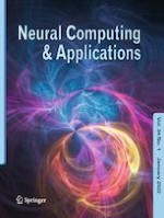
In case of complex data vectors, we realize the mapping \(\varPhi :\mathbb {C}^{n}\ni \mathbf {v}\rightarrow \left| \mathbf {x}\right\rangle \in \mathcal {H}^{n}\) by the nonlinear mapping \(\varphi \left( v_{l}\right) =\varPsi \circ \varPi \left( v_{l}\right) \) where \({{\varPi \left( z\right) }}\) is the stereographic projection of the complex number z
$$\begin{aligned} z\overset{\varPi }{\longmapsto }\mathbf {r}= & {} \left( r_{1},r_{2},r_{3}\right) \nonumber \\= & {} \left( \frac{z+\overline{z}}{1+\left| z\right| },\frac{z-\overline{z}}{i\cdot \left( 1+\left| z\right| \right) },\frac{\left| z\right| -1}{1+\left| z\right| }\right) \in \mathscr {R\subseteq \mathbb {R}}^{3} \end{aligned}$$
(32)
onto the Riemann sphere \(\mathscr {R}\) fulfilling the constraint \(\left\| \mathbf {r}\right\| =1\) for all \(\mathbf {r}\in \mathscr {R}\), see Fig. 1.
The subsequent mapping \(\varPsi \left( \mathbf {r}\right) \) delivers the spherical coordinates
$$\begin{aligned} \xi= & {} \arccos \left( r_{3}\right) \\ \\ \phi= & {} \arctan _{2}\left( \frac{r_{2}}{r_{1}}\right) \end{aligned}$$
of \(\mathbf {r}\) such that
$$\begin{aligned} \varphi \left( v_{l}\right) =\varPsi \left( \begin{array}{c} \xi \\ \phi \end{array}\right) \text { with }\left| x_{l}\right\rangle =\left[ \begin{array}{c} \cos \left( \xi \right) \\ \sin \left( \xi \right) \cdot \exp \left( i\cdot \phi \right) \end{array}\right] \end{aligned}$$
is obtained, see Fig. 2.
Note that the stereographic projection \(\varPi \left( z\right) \) is unique realizing a squashing effect. This effect becomes particularly apparent if \(\left| z\right| \rightarrow \infty \) and hence is comparable the squashing effect realized by \(\varPi \left( v_{l}\right) \) for the real case.

4 Numerical experiments

We tested the proposed Qu-GLVQ algorithm for several datasets in comparison with established LVQ approaches as well as SVM. Particularly, we compare Qu-GLVQ with standard GLVQ, KGLVQ and SVM. For both SVM and KGLVQ, the rbf-kernel was used with the same kernel width obtained by a grid search. For all LVQ variants including Qu-GLVQ, we used only one prototype per class for all experiments.
The datasets are a) WHISKY - a spectral dataset to classify Scottish whisky described in [1, 2], WBCD - UCI Wisconcin Breast Cancer Dataset, HEART - UCI Heart disease dataset, PIMA - UCI diabetes dataset, and FLC1 - satellite remote sensing LANDSAT TM dataset [27].2 The averaged results reported are obtained by 10-fold cross-validation. Only test accuracies are given.
Table 1
Classification accuracies in % and standard deviations for GLVQ, Qu-GLVQ, KGLVQ, and SVM for the considered datasets (10-fold cross-validation)
Dataset
N
d
\(\#C\)
GLVQ
Qu-GLVQ
KGLVQ
SVM
WHISKY
1188
401
3
92.5 ± 1.9
92.6 ± 1.4
86.9 ± 2.8
99.3 ± 0.7 (|SV|:140)
WBCD
569
30
2
96.8 ± 2.7
96.1 ± 3.4
94.0 ± 3.4
96.5 ± 1.5 (|SV|: 43)
HEART
297
13
2
56.9 ± 4.0
81.8 ± 5.3
84.3 ± 5.4
80.4 ± 9.5 (|SV|: 97)
FLC1
82045
12
10
92.8 ± 0.3
92.0 ± 0.4
94.8  ± 0.4
97.4 ± 0.1 (|SV|: 2206)
PIMA
768
8
2
77.3 ± 2.3
75.4 ± 2.4
76.4 ± 4.6
75.5 ± 4.1 (|SV|: 311)
Average
   
83.3 ± 2.2
87.6 ± 2.6
87.3 ± 3.3
89.8 ± 3.2
For all LVQ-algorithms, only one prototype per class was used. The number of support vectors for SVM is given by \(\left| SV\right| \). N number of data samples, d data dimensionality, \(\#C\) number of classes
We observe an overall good performance of QU-GLVQ comparable to the other methods, see Table 1. Kernel methods seem to be beneficial as indicated by KGLVQ and SVM for HEART. Yet, Qu-GLVQ delivers similar results. If SVM yields significant better performance than KLVQ and Qu-GLVQ, then we have to take into account that here the SVM complexity (number of support vectors) is much higher than in LVQ-networks, where the number of prototypes was chosen always to be only one per class. Further, for WHISKY the KGLVQ was not able to achieve a classification accuracy comparable to the other approaches, whereas Qu-GLVQ performed well. This might be addressed due to the crucial dependency of the rbf-kernel on the kernel width. Further, Qu-GLVQ seems to be more stable than KGLVQ and SVM considering the averaged deviations.

5 Conclusion

In this contribution, we introduced an approach to incorporate quantum machine learning strategies into the GLVQ framework. Usual data and prototype vectors are replaced by respective quantum bit vectors. This replacement can be seen as an explicit nonlinear mapping of the data into the quantum Hilbert space which make the difference to the implicit feature mapping in case of kernel methods like kernelized GLVQ or SVM. Thus, one can visualize and analyze the data as well as the prototypes in this space, such that Qu-GLVQ becomes better interpretable than KGLVQ or SVM without this possibility.
Otherwise, the QU-GLVQ approach shows mathematical equivalence to the kernel approaches in topological sense: the distance calculations are carried out in the mapping Hilbert space implicitly for usual kernels and explicitly for Qu-GLVQ. The resulting adaptation dynamic in Qu-GLVQ is consistent with the unitary transformations required for quantum state changes, because the prototypes remain quantum-state vectors.
Further investigations should include several modifications and extension of the proposed Qu-GLVQ. First, matrix learning like for GMLVQ can easily be integrated. Further, the influence of different transfer function as proposed in [62] for standard GLVQ has to be considered to improve learning speed and performance. A much more challenging task will be to consider entanglements for qubits and complex amplitudes \(\beta \in \mathbb {C}\) for qubits [20] in context of Qu-GLVQ. This research also should continue the approach in [71].
Finally, adaptation to a real quantum system is the final goal as recently realized for other classifier systems [47].
Overall, Qu-GLVQ performs equivalently to KGLVQ and SVM. However, due to its better interpretability it could be an interesting alternative if interpretable models are demanded.

Acknowledgements

AE, JR, and MK acknowledge support by a ESF Grant four young researchers. TV thanks Maria Schuld for stimulating discussions during NeurIPS 2019.

Compliance with ethical standards

Conflict of interest

The authors declare that they have no conflict of interest.
Open AccessThis article is licensed under a Creative Commons Attribution 4.0 International License, which permits use, sharing, adaptation, distribution and reproduction in any medium or format, as long as you give appropriate credit to the original author(s) and the source, provide a link to the Creative Commons licence, and indicate if changes were made. The images or other third party material in this article are included in the article's Creative Commons licence, unless indicated otherwise in a credit line to the material. If material is not included in the article's Creative Commons licence and your intended use is not permitted by statutory regulation or exceeds the permitted use, you will need to obtain permission directly from the copyright holder. To view a copy of this licence, visit http://​creativecommons.​org/​licenses/​by/​4.​0/​.

Publisher's Note

Springer Nature remains neutral with regard to jurisdictional claims in published maps and institutional affiliations.
Appendix

Appendix: Wirtinger calculus

In the following, we give a short introduction to the Wirtinger calculus [67]. We do not follow the complicate and old-fashioned notations in this original paper but prefer a more modern style. Thus, we follow [14].
We consider a real-valued function f of a complex argument \(z=x+\mathsf {i}y\)
$$\begin{aligned} f:\mathbb {C}\rightarrow \mathbb {R}\quad \text {with}\quad z=x+\mathsf {i}y\,\mapsto\, f\left( z\right) =u\left( x,y\right) \end{aligned}$$
with \(x,y\in \mathbb {R}\). Here, minimization of f is to be considered in dependence of the two real arguments x and y. For a complex-valued function g, we analogously have
$$\begin{aligned} g:\mathbb {C}\rightarrow \mathbb {C}\quad \text {with}\quad z=x+\mathsf {i}y\,\mapsto\, g\left( z\right) =u\left( x,y\right) +\mathsf {i}v\left( x,y\right) \end{aligned}$$
where \(v\left( x,y\right) \) is also real-valued. The differential operators of Wirtinger type are defined as
$$\begin{aligned} \frac{\partial _{\mathfrak {W}}}{\partial z}=\frac{1}{2}\left( \frac{\partial }{\partial x}-\mathsf {i}\frac{\partial }{\partial y}\right) \end{aligned}$$
(33)
and
$$\begin{aligned} \frac{\partial _{\mathfrak {W}}}{\partial \overline{z}}=\frac{1}{2}\left( \frac{\partial }{\partial x}+\mathsf {i}\frac{\partial }{\partial y}\right) \end{aligned}$$
(34)
where \(\frac{\partial }{\partial \overline{z}}\) is denoted as conjugate differential operator [67].
The respective calculus assumes differentiability of the functions f and g in the real-valued sense, i.e., the function \(u\left( x,y\right) \) and \(v\left( x,y\right) \) are assumed to be differentiable with respect to x and y. This Wirtinger-differentiability differs from usual differentiability of complex function, which requires the validity of the Cauchy-Riemann equation which reads as
$$\begin{aligned} \frac{\partial _{\mathfrak {W}}g}{\partial \overline{z}}=0 \end{aligned}$$
in terms of the Wirtinger calculus, i.e., the complex function is differentiable in z if the partial derivative \(\frac{\partial g}{\partial \overline{z}}\) vanishes.
Both, the product and the sum rule apply whereas the chain rule for a function \(h:\mathbb {R}\rightarrow \mathbb {R}\) becomes
$$\begin{aligned} \frac{\partial _{\mathfrak {W}}h\left( g\left( z\right) \right) }{\partial z}=\frac{\partial _{\mathfrak {W}}h}{\partial g}\frac{\partial _{\mathfrak {W}}g\left( z\right) }{\partial z}+\frac{\partial _{\mathfrak {W}}h}{\partial \overline{g}}\frac{\partial _{\mathfrak {W}}\overline{g}}{\partial z} \end{aligned}$$
and likewise for the conjugate derivative for \(\overline{z}\). If a function f is given in the form \(f\left( z,\overline{z}\right) \) then in \(\frac{\partial _{\mathfrak {W}}f}{\partial z}\) the variable \(\overline{z}\) is treated as constant and vice versa. For example, we have for \(f\left( z\right) =\left| z\right| ^{2}\) the derivatives \(\frac{\partial _{\mathfrak {W}}f}{\partial z}=\overline{z}\) and \(\frac{\partial _{\mathfrak {W}}f}{\partial \overline{z}}=z\) because of \(\left| z\right| ^{2}=z\cdot \overline{z}\). Yet, \(\frac{\partial _{\mathfrak {W}}z^{2}}{\partial z}=2z\) is equivalent to the real case.
Next we consider complex vectors \(\mathbf {z}\in \mathbb {C}^{n}\). The squared Euclidean norm is \(\left\| \mathbf {z}\right\| _{2}^{2}=\mathbf {z}^{*}\mathbf {z}\), where \(\mathbf {z}^{*}\) denotes the Hermitian transpose. We immediately obtain
$$\begin{aligned} \frac{\partial _{\mathfrak {W}}\left\| \mathbf {z}\right\| _{2}^{2}}{\partial \mathbf {z}}=\mathbf {z}^{*}\quad \text {and}\quad \frac{\partial _{\mathfrak {W}}\left\| \mathbf {z}\right\| _{2}^{2}}{\partial \mathbf {z}^{*}}=\mathbf {z} \end{aligned}$$
whereas for the quadratic form \(\left\| \mathbf {z}\right\| _{\mathbf {A},2}^{2}=\mathbf {z}^{*}\mathbf {A}\mathbf {z}\) with \(\mathbf {A}\in \mathbb {C}^{n\times n}\) we obtain
$$\begin{aligned} \frac{\partial _{\mathfrak {W}}\left\| \mathbf {z}\right\| _{\mathbf {A},2}^{2}}{\partial \mathbf {z}}=\mathbf {A}^{*}\mathbf {z}^{*}\quad \text {and}\quad \frac{\partial _{\mathfrak {W}}\left\| \mathbf {z}\right\| _{\mathbf {A},2}^{2}}{\partial \mathbf {z}^{*}}=\mathbf {A}\mathbf {z} \end{aligned}$$
as Wirtinger derivatives.
Footnotes
1
This assumption reduces the Bloch-sphere to a circle. With other words, here the phase information is set to \(e^{i\phi }\) with \(\phi =0\).
 
2
The UCI-datasets are available from: https://​archive.​ics.​uci.​edu/​ml.
 
Literature
1.
go back to reference Ashok P, Praveen B, Dholakia K (2011) Near infrared spectroscopic analysis of single malt Scotch whisky on an optofluidic chip. Opt Express 19(23):1–11 Ashok P, Praveen B, Dholakia K (2011) Near infrared spectroscopic analysis of single malt Scotch whisky on an optofluidic chip. Opt Express 19(23):1–11
2.
go back to reference Backhaus A, Ashok P, Praveen B, Dholakia K, Seiffert U (2012) Classifying scotch whisky from near-infrared Raman spectra with a radial basis function network with relevance learning. In: Verleysen M (ed) Proceedings of the European symposium on artificial neural networks and machine learning (ESANN), pp 411–416. i6doc.com, Brussels Backhaus A, Ashok P, Praveen B, Dholakia K, Seiffert U (2012) Classifying scotch whisky from near-infrared Raman spectra with a radial basis function network with relevance learning. In: Verleysen M (ed) Proceedings of the European symposium on artificial neural networks and machine learning (ESANN), pp 411–416. i6doc.com, Brussels
3.
go back to reference Biamonte J, Wittek P, Pancotti N, Rebentrost P, Wiebe N, Lloyd S (2017) Quantum machine learning. Nature 549(9):195–202 Biamonte J, Wittek P, Pancotti N, Rebentrost P, Wiebe N, Lloyd S (2017) Quantum machine learning. Nature 549(9):195–202
4.
go back to reference Biehl M, Hammer B, Villmann T (2016) Prototype-based models in machine learning. Wiley Interdiscip Rev Cognit Sci 2:92–111 Biehl M, Hammer B, Villmann T (2016) Prototype-based models in machine learning. Wiley Interdiscip Rev Cognit Sci 2:92–111
5.
go back to reference Bishop C (2006) Pattern recognition and machine learning. Springer, BerlinMATH Bishop C (2006) Pattern recognition and machine learning. Springer, BerlinMATH
6.
go back to reference Bouboulis P, Theododoridis S (2011) Extension of Wirtinger’s calculus to reproducing kernel Hilbert spaces and the complex LMS. IEEE Trans Signal Process 59(3):964–978MathSciNetMATH Bouboulis P, Theododoridis S (2011) Extension of Wirtinger’s calculus to reproducing kernel Hilbert spaces and the complex LMS. IEEE Trans Signal Process 59(3):964–978MathSciNetMATH
7.
go back to reference Bouboulis P, Theododoridis S, Mavroforakis C, Evaggelatou-Dalla L (2015) Complex support vector machines for regression and quaternary classification. IEEE Trans Neural Netw Learn Syst 26(6):1260–1274MathSciNet Bouboulis P, Theododoridis S, Mavroforakis C, Evaggelatou-Dalla L (2015) Complex support vector machines for regression and quaternary classification. IEEE Trans Neural Netw Learn Syst 26(6):1260–1274MathSciNet
8.
go back to reference Bunte K, Schneider P, Hammer B, Schleif FM, Villmann T, Biehl M (2012) Limited rank matrix learning, discriminative dimension reduction and visualization. Neural Netw 26(1):159–173 Bunte K, Schneider P, Hammer B, Schleif FM, Villmann T, Biehl M (2012) Limited rank matrix learning, discriminative dimension reduction and visualization. Neural Netw 26(1):159–173
9.
go back to reference Ciliberto C, Herbster M, Ialongo A, Pontil M, Rocchetto A, Severini S, Wossnig L (2018) Quantum machine learning: a classical perspective. Proc R Soc A 474(2209):1–26MathSciNetMATH Ciliberto C, Herbster M, Ialongo A, Pontil M, Rocchetto A, Severini S, Wossnig L (2018) Quantum machine learning: a classical perspective. Proc R Soc A 474(2209):1–26MathSciNetMATH
10.
go back to reference Crammer K, Gilad-Bachrach R, Navot A, Tishby A (2003) Margin analysis of the LVQ algorithm. In: Becker S, Thrun S, Obermayer K (eds) Advances in neural information processing (Proceedings of the NIPS 2002), vol 15, pp 462–469. MIT Press, Cambridge, MA Crammer K, Gilad-Bachrach R, Navot A, Tishby A (2003) Margin analysis of the LVQ algorithm. In: Becker S, Thrun S, Obermayer K (eds) Advances in neural information processing (Proceedings of the NIPS 2002), vol 15, pp 462–469. MIT Press, Cambridge, MA
11.
go back to reference Cristianini N, Shawe-Taylor J (2000) An introduction to support vector machines and other kernel-based learning methods. Cambridge University Press, CambridgeMATH Cristianini N, Shawe-Taylor J (2000) An introduction to support vector machines and other kernel-based learning methods. Cambridge University Press, CambridgeMATH
12.
go back to reference Dunjko V, Taylor J, Briegel H (2016) Quantum-enhanced machine learning. Phys Rev Lett 117(130501):1–6MathSciNet Dunjko V, Taylor J, Briegel H (2016) Quantum-enhanced machine learning. Phys Rev Lett 117(130501):1–6MathSciNet
13.
go back to reference Eisenreich G (1980) Lineare Algebra und analytische Geometrie. Akademie-Verlag, BerlinMATH Eisenreich G (1980) Lineare Algebra und analytische Geometrie. Akademie-Verlag, BerlinMATH
14.
go back to reference Gay M, Kaden M, Biehl M, Lampe A, Villmann T (2016) Complex variants of GLVQ based on Wirtinger’s calculus. In: Merényi E, Mendenhall M, O’Driscoll P (eds) Advances in self-organizing maps and learning vector quantization—Proceedings of 11th international workshop WSOM 2016. Advances in intelligent systems and computing, vol 428, pp 293–303. Springer, Berlin Gay M, Kaden M, Biehl M, Lampe A, Villmann T (2016) Complex variants of GLVQ based on Wirtinger’s calculus. In: Merényi E, Mendenhall M, O’Driscoll P (eds) Advances in self-organizing maps and learning vector quantization—Proceedings of 11th international workshop WSOM 2016. Advances in intelligent systems and computing, vol 428, pp 293–303. Springer, Berlin
15.
go back to reference Goodfellow I, Bengio Y, Courville A (2016) Deep learning. MIT Press, CambridgeMATH Goodfellow I, Bengio Y, Courville A (2016) Deep learning. MIT Press, CambridgeMATH
16.
go back to reference Havlicek V, Corcoles A, Temme K, Harrow A, Kandala A, Chow J, Gambetta J (2019) Supervised learning with quantum-enhanced feature spaces. Nature 567(3):209–212 Havlicek V, Corcoles A, Temme K, Harrow A, Kandala A, Chow J, Gambetta J (2019) Supervised learning with quantum-enhanced feature spaces. Nature 567(3):209–212
17.
go back to reference Hoffmann T, Schölkopf B, Smola A (2008) Kernel methods in machine learning. Ann Stat 36(3):1171–1220MathSciNetMATH Hoffmann T, Schölkopf B, Smola A (2008) Kernel methods in machine learning. Ann Stat 36(3):1171–1220MathSciNetMATH
18.
go back to reference Hou X (2011) Research of model of quantum learning vector quantization neural network. In: Proceedings of the international conference on electronic and mechanical engineering and information technology, pp 3893–3896. IEEE Society, Los Alamitos Hou X (2011) Research of model of quantum learning vector quantization neural network. In: Proceedings of the international conference on electronic and mechanical engineering and information technology, pp 3893–3896. IEEE Society, Los Alamitos
19.
go back to reference Hu W (2018) Comparison of two quantum nearest neighbor classifiers on IBM’s quantum simulator. Nat Sci 10(3):87–98 Hu W (2018) Comparison of two quantum nearest neighbor classifiers on IBM’s quantum simulator. Nat Sci 10(3):87–98
20.
go back to reference Huusari R, Kadri H (2019) Entangled kernels. In: Kraus S (ed) Proceedings of the 28th international joint conference on artificial intelligence (IJCAI-19), Macao, pp 2578–2584. International Joint Conferences on Artificial Intelligence Huusari R, Kadri H (2019) Entangled kernels. In: Kraus S (ed) Proceedings of the 28th international joint conference on artificial intelligence (IJCAI-19), Macao, pp 2578–2584. International Joint Conferences on Artificial Intelligence
21.
go back to reference Kaden M, Bohnsack K, Weber M, Kudla M, Gutoska K, Blasewicz J, Villmann T (2020) Analysis of SARS-CoV-2 RNA-sequences by interpretable machine learning models. Technical Report, arXiv:1901.05995 Kaden M, Bohnsack K, Weber M, Kudla M, Gutoska K, Blasewicz J, Villmann T (2020) Analysis of SARS-CoV-2 RNA-sequences by interpretable machine learning models. Technical Report, arXiv:​1901.​05995
22.
go back to reference Kerenidis I, Landman J, Luongo A, Prakash A (2019) q-means: a quantum algorithm for unsupervised machine learning. In: Wallach H, Larochelle H, Beygelzimer A, dAlché Buc F, Fox E, Garnett R (eds) Advances in neural information processing systems 32 (NIPS 2019), pp 4134–4144. Curran Associates, Inc Kerenidis I, Landman J, Luongo A, Prakash A (2019) q-means: a quantum algorithm for unsupervised machine learning. In: Wallach H, Larochelle H, Beygelzimer A, dAlché Buc F, Fox E, Garnett R (eds) Advances in neural information processing systems 32 (NIPS 2019), pp 4134–4144. Curran Associates, Inc
23.
go back to reference Kohonen T (1988) Learning vector quantization. Neural Netw 1(Supplement 1):303 Kohonen T (1988) Learning vector quantization. Neural Netw 1(Supplement 1):303
24.
go back to reference Kohonen T (1990) Improved versions of learning vector quantization. In: Proceedings of the IJCNN-90. International joint conference on neural networks, San Diego, vol I, pp 545–550. IEEE Service Center, Piscataway, NJ Kohonen T (1990) Improved versions of learning vector quantization. In: Proceedings of the IJCNN-90. International joint conference on neural networks, San Diego, vol I, pp 545–550. IEEE Service Center, Piscataway, NJ
25.
go back to reference Kohonen T (1995) Self-organizing maps. Springer Series in Information Sciences, vol 30. Springer, Berlin (second extended edition 1997) Kohonen T (1995) Self-organizing maps. Springer Series in Information Sciences, vol 30. Springer, Berlin (second extended edition 1997)
26.
go back to reference Lamata L (2020) Quantum machine learning and quantum biomimetics: a perspective. Mach Learn Sci Technol 1(3–03300):1–11 Lamata L (2020) Quantum machine learning and quantum biomimetics: a perspective. Mach Learn Sci Technol 1(3–03300):1–11
27.
go back to reference Landgrebe D (2003) Signal theory methods in multispectral remote sensing. Wiley, Hoboken Landgrebe D (2003) Signal theory methods in multispectral remote sensing. Wiley, Hoboken
28.
go back to reference LeCun Y, Bengio Y, Hinton G (2015) Deep learning. Nature 52:1097–1105 LeCun Y, Bengio Y, Hinton G (2015) Deep learning. Nature 52:1097–1105
29.
go back to reference Li O, Liu H, Chen C, Rudin C (2018) Deep learning for case-based reasoning through prototypes: a neural network that explains its predictions. In: Proceedings of the 32nd AAAI conference on artificial intelligence (AAAI-18), pp 3531–3537. Association for the Advancement of Artificial Intelligence, AAAI Press Li O, Liu H, Chen C, Rudin C (2018) Deep learning for case-based reasoning through prototypes: a neural network that explains its predictions. In: Proceedings of the 32nd AAAI conference on artificial intelligence (AAAI-18), pp 3531–3537. Association for the Advancement of Artificial Intelligence, AAAI Press
30.
go back to reference Lindner A (2018) A complete course on theoretical physics. Springer Nature Switzerland AG, Springer, ChamMATH Lindner A (2018) A complete course on theoretical physics. Springer Nature Switzerland AG, Springer, ChamMATH
31.
go back to reference Mwebaze E, Schneider P, Schleif FM, Aduwo J, Quinn J, Haase S, Villmann T, Biehl M (2011) Divergence based classification in learning vector quantization. Neurocomputing 74(9):1429–1435 Mwebaze E, Schneider P, Schleif FM, Aduwo J, Quinn J, Haase S, Villmann T, Biehl M (2011) Divergence based classification in learning vector quantization. Neurocomputing 74(9):1429–1435
32.
go back to reference Nebel D, Hammer B, Frohberg K, Villmann T (2015) Median variants of learning vector quantization for learning of dissimilarity data. Neurocomputing 169:295–305 Nebel D, Hammer B, Frohberg K, Villmann T (2015) Median variants of learning vector quantization for learning of dissimilarity data. Neurocomputing 169:295–305
33.
go back to reference Nielsen M, Chuang I (2016) Quantum computation and quantum information, 10th edn. Cambridge University Press, CambridgeMATH Nielsen M, Chuang I (2016) Quantum computation and quantum information, 10th edn. Cambridge University Press, CambridgeMATH
34.
go back to reference Oehler KL, Gray RM (1995) Combining image compression and classification using vector quantization. IEEE Trans Pattern Anal Mach Intell 17:461–473 Oehler KL, Gray RM (1995) Combining image compression and classification using vector quantization. IEEE Trans Pattern Anal Mach Intell 17:461–473
35.
go back to reference Rebentrost P, Bromley T, Weedbrook C, Lloyd S (2018) Quantum Hopfield neural network. Phys Rev A 98(042308):1–11 Rebentrost P, Bromley T, Weedbrook C, Lloyd S (2018) Quantum Hopfield neural network. Phys Rev A 98(042308):1–11
36.
go back to reference Rebentrost P, Mohseni M, Lloyd S (2014) Quantum support vector machines for big data classification. Phys Rev Lett 113(13050):1–5 Rebentrost P, Mohseni M, Lloyd S (2014) Quantum support vector machines for big data classification. Phys Rev Lett 113(13050):1–5
37.
go back to reference Ritter H, Martinetz T, Schulten K (1992) Neural computation and self-organizing maps: an introduction. Addison-Wesley, ReadingMATH Ritter H, Martinetz T, Schulten K (1992) Neural computation and self-organizing maps: an introduction. Addison-Wesley, ReadingMATH
38.
39.
go back to reference Rudin C (2019) Stop explaining black box machine learning models for high stakes decisions and use interpretable models instead. Nat Mach Intell 1(5):206–215 Rudin C (2019) Stop explaining black box machine learning models for high stakes decisions and use interpretable models instead. Nat Mach Intell 1(5):206–215
40.
go back to reference Samek W, Monatvon G, Vedaldi A, Hansen L, Müller KR (eds) (2019) Explainable AI: interpreting, explaining and visualizing deep learning, No 11700 in LNAI. Springer Samek W, Monatvon G, Vedaldi A, Hansen L, Müller KR (eds) (2019) Explainable AI: interpreting, explaining and visualizing deep learning, No 11700 in LNAI. Springer
41.
go back to reference Saralajew S, Holdijk L, Rees M, Villmann T (2019) Robustness of generalized learning vector quantization models against adversarial attacks. In: Vellido A, Gibert K, Angulo C, Guerrero J (eds) Advances in self-organizing maps, learning vector quantization, clustering and data visualization—Proceedings of the 13th international workshop on self-organizing maps and learning vector quantization, clustering and data visualization, WSOM+2019, Barcelona. Advances in intelligent systems and computing, vol 976, pp 189–199. Springer, Berlin Saralajew S, Holdijk L, Rees M, Villmann T (2019) Robustness of generalized learning vector quantization models against adversarial attacks. In: Vellido A, Gibert K, Angulo C, Guerrero J (eds) Advances in self-organizing maps, learning vector quantization, clustering and data visualization—Proceedings of the 13th international workshop on self-organizing maps and learning vector quantization, clustering and data visualization, WSOM+2019, Barcelona. Advances in intelligent systems and computing, vol 976, pp 189–199. Springer, Berlin
42.
go back to reference Sato A, Yamada K (1996) Generalized learning vector quantization. In: Touretzky DS, Mozer MC, Hasselmo ME (eds) Proceedings of the 1995 conference on advances in neural information processing systems 8, pp 423–429. MIT Press, Cambridge, MA, USA Sato A, Yamada K (1996) Generalized learning vector quantization. In: Touretzky DS, Mozer MC, Hasselmo ME (eds) Proceedings of the 1995 conference on advances in neural information processing systems 8, pp 423–429. MIT Press, Cambridge, MA, USA
43.
go back to reference Schneider P, Hammer B, Biehl M (2009) Adaptive relevance matrices in learning vector quantization. Neural Comput 21:3532–3561MathSciNetMATH Schneider P, Hammer B, Biehl M (2009) Adaptive relevance matrices in learning vector quantization. Neural Comput 21:3532–3561MathSciNetMATH
44.
go back to reference Schneider P, Hammer B, Biehl M (2009) Distance learning in discriminative vector quantization. Neural Comput 21:2942–2969MathSciNetMATH Schneider P, Hammer B, Biehl M (2009) Distance learning in discriminative vector quantization. Neural Comput 21:2942–2969MathSciNetMATH
45.
go back to reference Schölkopf B, Smola A (2002) Learning with kernels. MIT Press, CambridgeMATH Schölkopf B, Smola A (2002) Learning with kernels. MIT Press, CambridgeMATH
46.
go back to reference Schuld M (2019) Machine learning in quantum spaces. Nature 567:179–181 Schuld M (2019) Machine learning in quantum spaces. Nature 567:179–181
47.
go back to reference Schuld M, Bocharov A, Svore K, Wiebe N (2020) Circuit-centric quantum classifiers. Phys Rev A 101(032308):1–8MathSciNet Schuld M, Bocharov A, Svore K, Wiebe N (2020) Circuit-centric quantum classifiers. Phys Rev A 101(032308):1–8MathSciNet
48.
go back to reference Schuld M, Killoran N (2019) Quantum machine learning in feature Hilbert spaces. Phys Rev Lett 122(040504):1–6 Schuld M, Killoran N (2019) Quantum machine learning in feature Hilbert spaces. Phys Rev Lett 122(040504):1–6
49.
go back to reference Schuld M, Sinayskiy I, Petruccione F (2014) An introduction to quantum machine learning. Contemp Phys 56:172–185MATH Schuld M, Sinayskiy I, Petruccione F (2014) An introduction to quantum machine learning. Contemp Phys 56:172–185MATH
50.
go back to reference Scott T, Therani M, Wang X (2017) Data clustering with quantum mechanics. Mathematics 5(5):1–17MATH Scott T, Therani M, Wang X (2017) Data clustering with quantum mechanics. Mathematics 5(5):1–17MATH
51.
go back to reference Shawe-Taylor J, Cristianini N (2004) Kernel methods for pattern analysis and discovery. Cambridge University Press, CambridgeMATH Shawe-Taylor J, Cristianini N (2004) Kernel methods for pattern analysis and discovery. Cambridge University Press, CambridgeMATH
52.
go back to reference Steinwart I (2001) On the influence of the kernel on the consistency of support vector machines. J Mach Learn Res 2:67–93MathSciNetMATH Steinwart I (2001) On the influence of the kernel on the consistency of support vector machines. J Mach Learn Res 2:67–93MathSciNetMATH
53.
go back to reference Steinwart I, Christmann A (2008) Support vector machines. information science and statistics. Springer, BerlinMATH Steinwart I, Christmann A (2008) Support vector machines. information science and statistics. Springer, BerlinMATH
55.
go back to reference Tang E (2019) A quantum-inspired classical algorithm for recommendation systems. In: Proceedings of the 51st annual ACM SIGACT symposium on theory of computing-STOC 2019, pp 217–228. Association for Computing Machinery, New York, NY, USA Tang E (2019) A quantum-inspired classical algorithm for recommendation systems. In: Proceedings of the 51st annual ACM SIGACT symposium on theory of computing-STOC 2019, pp 217–228. Association for Computing Machinery, New York, NY, USA
57.
go back to reference Villmann T, Bohnsack A, Kaden M (2017) Can learning vector quantization be an alternative to SVM and deep learning? J Artif Intell Soft Comput Res 7(1):65–81 Villmann T, Bohnsack A, Kaden M (2017) Can learning vector quantization be an alternative to SVM and deep learning? J Artif Intell Soft Comput Res 7(1):65–81
58.
59.
go back to reference Villmann T, Haase S, Kaden M (2015) Kernelized vector quantization in gradient-descent learning. Neurocomputing 147:83–95 Villmann T, Haase S, Kaden M (2015) Kernelized vector quantization in gradient-descent learning. Neurocomputing 147:83–95
60.
go back to reference Villmann T, Kästner M, Nebel D, Riedel M (2014) Lateral enhancement in adaptative metric learning for functional data. Neurocomputing 131:23–31 Villmann T, Kästner M, Nebel D, Riedel M (2014) Lateral enhancement in adaptative metric learning for functional data. Neurocomputing 131:23–31
61.
go back to reference Villmann T, Ravichandran J, Engelsberger A, Villmann A, Kaden M (2020) Quantum-inspired learning vector quantization for classification learning. In: Verleysen M (ed) Proceedings of the 28th European symposium on artificial neural networks, computational intelligence and machine learning (ESANN’2020), Bruges (Belgium), pp 279–284. i6doc.com, Louvain-La-Neuve, Belgium Villmann T, Ravichandran J, Engelsberger A, Villmann A, Kaden M (2020) Quantum-inspired learning vector quantization for classification learning. In: Verleysen M (ed) Proceedings of the 28th European symposium on artificial neural networks, computational intelligence and machine learning (ESANN’2020), Bruges (Belgium), pp 279–284. i6doc.com, Louvain-La-Neuve, Belgium
62.
go back to reference Villmann T, Ravichandran J, Villmann A, Nebel D, Kaden M (2019) Investigation of activation functions for generalized learning vector quantization. In: Vellido A, Gibert K, Angulo C, Guerrero J (eds) Advances in self-organizing maps, learning vector quantization, clustering and data visualization—Proceedings of the 13th international workshop on self-organizing maps and learning vector quantization, clustering and data visualization, WSOM+2019, Barcelona. Advances in Intelligent systems and computing, vol 976, pp 179–188. Springer, Berlin Villmann T, Ravichandran J, Villmann A, Nebel D, Kaden M (2019) Investigation of activation functions for generalized learning vector quantization. In: Vellido A, Gibert K, Angulo C, Guerrero J (eds) Advances in self-organizing maps, learning vector quantization, clustering and data visualization—Proceedings of the 13th international workshop on self-organizing maps and learning vector quantization, clustering and data visualization, WSOM+2019, Barcelona. Advances in Intelligent systems and computing, vol 976, pp 179–188. Springer, Berlin
63.
go back to reference Villmann T, Saralajew S, Villmann A, Kaden M (2018) Learning vector quantization methods for interpretable classification learning and multilayer networks. In: Sabourin C, Merelo J, Barranco A, Madani K, Warwick K (eds) Proceedings of the 10th international joint conference on computational intelligence (IJCCI), Sevilla, pp 15–21. SCITEPRESS—Science and Technology Publications, Lda, Lissabon, Portugal Villmann T, Saralajew S, Villmann A, Kaden M (2018) Learning vector quantization methods for interpretable classification learning and multilayer networks. In: Sabourin C, Merelo J, Barranco A, Madani K, Warwick K (eds) Proceedings of the 10th international joint conference on computational intelligence (IJCCI), Sevilla, pp 15–21. SCITEPRESS—Science and Technology Publications, Lda, Lissabon, Portugal
64.
go back to reference Wan K, Dahlsten O, Kristjánsson H, Kim M (2017) Quantum generalisation of feedforward neural networks. npj Quantum Inf 3(6):1–8 Wan K, Dahlsten O, Kristjánsson H, Kim M (2017) Quantum generalisation of feedforward neural networks. npj Quantum Inf 3(6):1–8
65.
go back to reference Wiebe N, Kapoor A, Svore K (2015) Quantum algortihms for nearest-neighbor methods for supervised and unsupervised learning. Quantum Inf Comput 15(3–4):0316–0356MathSciNet Wiebe N, Kapoor A, Svore K (2015) Quantum algortihms for nearest-neighbor methods for supervised and unsupervised learning. Quantum Inf Comput 15(3–4):0316–0356MathSciNet
66.
go back to reference Wiebe N, Kapoor A, Svore K (2016) Quantum perceptron models. In: Lee DD, Sugiyama M, Luxburg UV, Guyon I, Garnett R (eds) Advances in neural information processing systems 29, pp 3999–4007. Curran Associates, Inc Wiebe N, Kapoor A, Svore K (2016) Quantum perceptron models. In: Lee DD, Sugiyama M, Luxburg UV, Guyon I, Garnett R (eds) Advances in neural information processing systems 29, pp 3999–4007. Curran Associates, Inc
67.
go back to reference Wirtinger W (1926) Zur formalen Theorie der Funktionen von mehr komplexen Veränderlichen. Math Ann 97:357–375MathSciNetMATH Wirtinger W (1926) Zur formalen Theorie der Funktionen von mehr komplexen Veränderlichen. Math Ann 97:357–375MathSciNetMATH
68.
go back to reference Wittek P (2014) Quantum machine learning—what quantum computing means to data mining, 1st edn. Elsevier, AmsterdamMATH Wittek P (2014) Quantum machine learning—what quantum computing means to data mining, 1st edn. Elsevier, AmsterdamMATH
69.
go back to reference Xiao-Yan Z, Xing-Xing A, Wen-Jie L, Fu-Gao J (2017) Quantum k-means algorithm based on the minimum distance. J Chin Comput Sci 38(5):1059–1062 Xiao-Yan Z, Xing-Xing A, Wen-Jie L, Fu-Gao J (2017) Quantum k-means algorithm based on the minimum distance. J Chin Comput Sci 38(5):1059–1062
70.
go back to reference Zeng J, Ustun B, Rudin C (2017) Interpretable classification models for recidivism prediction. J R Stat Soc Ser A 180:1–34MathSciNet Zeng J, Ustun B, Rudin C (2017) Interpretable classification models for recidivism prediction. J R Stat Soc Ser A 180:1–34MathSciNet
71.
go back to reference Zidan M, Abdel-Aty A, El-Shafei M, Feraig M, Al-Sbou Y, Eleuch H, Abdel-Aty M (2019) Quantum classification algorithm based on competitive learning neural network and entanglement measure. MDPI Appl Sci 9:1–15 Zidan M, Abdel-Aty A, El-Shafei M, Feraig M, Al-Sbou Y, Eleuch H, Abdel-Aty M (2019) Quantum classification algorithm based on competitive learning neural network and entanglement measure. MDPI Appl Sci 9:1–15
Metadata
Title
Quantum-inspired learning vector quantizers for prototype-based classification
Confidential: for personal use only—submitted to Neural Networks and Applications 5/2020
Authors
Thomas Villmann
Alexander Engelsberger
Jensun Ravichandran
Andrea Villmann
Marika Kaden
Publication date
24-11-2020
Publisher
Springer London
Published in
Neural Computing and Applications / Issue 1/2022
Print ISSN: 0941-0643
Electronic ISSN: 1433-3058
DOI
https://doi.org/10.1007/s00521-020-05517-y

Other articles of this Issue 1/2022

Neural Computing and Applications 1/2022 Go to the issue

Premium Partner