Answer set programming (ASP) is a declarative programming paradigm where the solutions of a search problem are captured by the answer sets of a logic program describing its solutions. Besides native algorithms implemented as answer-set solvers, the computation of answer sets can be realized (i) by translating the logic program into propositional logic or its extensions and (ii) by finding satisfying assignments with appropriate solvers. In this work, we recall the graph-based extension of propositional logic, viz. SAT modulo graphs, and the case of acyclicity constraint which keeps a digraph associated with each truth assignment acyclic. This particular extension lends itself very well for answer set computation, e.g., using extended SAT solvers, such as GraphSAT, as back-end solvers. The goal of this work, however, is to translate away the acyclicity extension altogether using a vertex elimination technique, giving rise to a translation from ASP into propositional clauses only. We use non-tight benchmarks and a state-of-the-art SAT solver, Kissat, to illustrate that performance obtained in this way can be competitive against GraphSAT and native ASP solvers such as Clasp and Wasp.
Hinweise
The original version of this chapter was revised: this chapter was previously published non-open access. The correction to this chapter is available at https://doi.org/10.1007/978-3-031-15707-3_40
1 Introduction
Answer set programming (ASP) is a paradigm for declarative programming where the solutions of a search problem are described in terms of rules (see, e.g., [6, 15] for overviews). A central idea behind the paradigm is that the solutions of the problem are captured by the answer sets [16] of the logic program formed by the rules. Then, solutions can be sought using dedicated search engines, known as answer-set solvers, for the computation of answer sets. The performance of answer-set solvers has been evaluated in a series of ASP competitions, see [12] for the results of the seventh competition. The latest competitions have been dominated by native answer-set solvers Clasp [11] and Wasp [1], making them as natural targets for comparison when improving answer set computation.
Besides native native answer-set solvers, the computation of answer sets can be realized via translations into propositional (Boolean) logic such that Boolean satisfiability (SAT) checkers, also known as SAT solvers, can be used to find satisfying assignments corresponding to answer sets. Such a strategy for answer set computation is more generally known as translation-based ASP [14] that was originally proposed to combine the knowledge representation capabilities of ASP with the efficiency of existing solver technology. There is some variety of translations from ASP to pure SAT, including worst-case exponential [18], quadratic [17], and sub-quadratic [13] ones. Yet more compact (linear) translations are enabled if one considers extensions of propositional logic such as difference logic (DL) [20] and SAT modulo graphs [9]. The latter is particularly relevant for the purposes of this work in the case of acyclicity constraint which keeps a digraph associated with each truth assignment acyclic. This primitive is well-suited for expressing the essentials of answer sets [8] as well as for their computation, e.g., using extended SAT solvers, such as GraphSAT [10], as back-ends. As reflected by ASP competition results, the level of performance obtained via translations can be sometimes comparable to that of native solvers, but no translation-based approach has really been able to challenge native ASP solvers so far. At best, non-native back-end solvers scale similarly, but the performance is degraded by slower propagation due to blow-ups and primitives used in translation.
Anzeige
In this work, however, we take advantage of a recently introduced method that translates away the acyclicity constraints altogether using a vertex elimination technique [21]. Our translation is therefore from ASP into pure SAT. While GraphSAT relies on a specialized algorithm for satisfying the acyclicity constraint, our method offers an easy way to use any state-of-the-art SAT solver as the back-end solver without additional implementation effort.
Our translation of ASP into pure SAT is produced through four stages, which respectively are normalization, instrumentation with acyclicity constraint, program completion, and translating the acyclicity constraint to propositional clauses using vertex elimination. We theoretically show how the correctness of our method can be derived from the correctness of the mentioned stages. As for the empirical analysis, by considering non-tight decision problem sets of previous ASP competitions, we show that our new translation-based method, when accompanied by a state-of-the-art SAT solver, Kissat [2], outperforms previous translation-based methods, and is also quite competitive against state-of-the-art native ASP solvers such as Clasp and Wasp. To the best of our knowledge and referring to ASP Competition results, this is the first time when a translation-based approach to answer-set solving has actualized its intended potential.
The rest of this article is organized as follows. In Sect. 2, we recall basic concepts and definitions of ASP and identify the class of weight constraint programs (WCPs) that is central for this study. Then, in Sect. 3, we discuss the three basic steps required to transform a WCP P into a set of clauses amended by a dynamically varying digraph that is enforced to be acyclic. In Sect. 4, we recall how vertex elimination can be used to check whether a given digraph is acyclic. Then, we describe how SAT modulo acyclicity can be translated back to pure SAT using vertex elimination in Sect. 5. In Sect. 6, we combine the techniques presented so far and present a novel translation of WCPs into pure SAT, improving the efficiency of computing answer sets with SAT solvers. To this end, we present practical evidence in Sect. 7 based on an experimental evaluation of the resulting method for answer set computation. The analysis is based on six non-tight benchmark problems. Finally, we conclude the paper in Sect. 8.
2 Preliminaries
In the sequel, weight constraint programs (WCPs) consist of rules of the forms:
The symbols a, \({b_1}\,{,}\ldots {,}\,{b_n}\) with \(n\ge 0\), and \({c_1}\,{,}\ldots {,}\,{c_m}\) with \(m\ge 0\) occurring in the rules are (propositional) atoms and “\(\texttt{not}\,\,\!\!\)” denotes negation by default. The boundk and the weights\({w_1}\,{,}\ldots {,}\,{w_{n+m}}\) in (3) are non-negative integers. Rules of the forms (1)–(3) are known as normal, choice, and weightrules, respectively [23]. Intuitively, each rule r gives a reason to derive its head\(\textrm{head}(r)=a\) if the conditions in its body\(\textrm{body}(r)\) are met, i.e., atoms involved can be either derived or not by other rules. For a choice rule r of form (2), the derivation of \(\textrm{head}(r)\) is optional and, for a weight rule r of form (3), the sum of weights associated with satisfied body conditions must reach k. We write \(\textrm{body}^+(r)\) and \(\textrm{body}^-(r)\) for the sets of atoms \({b_1}\,{,}\ldots {,}\,{b_n}\) (resp. \({c_1}\,{,}\ldots {,}\,{c_m}\)) occurring positively (resp. negatively) in \(\textrm{body}(r)\). A normal logic program (NLP) consists of normal rules only whereas the rules of a positive logic program satisfy \(m=0\), i.e., are negation free. Given a WCP P, the definition of an atom a in P is \(\textrm{def}_{P}(a)=\{{r\,\in \, P}\mid {\textrm{head}(r)=a}\}\).
Anzeige
The signature of a WCP P is the set of atoms \(\textrm{At}(P)=\bigcup _{r\,\in \, P}(\{\textrm{head}(r)\}\cup \textrm{body}^+(r)\cup \textrm{body}^-(r))\) that occur in P. The positive dependency graph of P is \(\textrm{DG}^+(P)\langle {\textrm{At}(P),\mathbin {\succeq }}\rangle \) where \(a\mathbin {\succeq }b\) holds for \(a,b\,\in \,\textrm{At}(P)\) if \(\textrm{head}(r)=a\) and \(b\,\in \,\textrm{body}^+(r)\) for some rule \(r\,\in \, P\). A strongly connected component (SCC) of \(\textrm{DG}^+(P)\) is a maximal subset \(S\subseteq \textrm{At}(P)\) such that all distinct atoms \(a,b\,\in \, S\) depend (transitively) on each other via a directed path in \(\textrm{DG}^+(P)\).
An interpretation\(I\subseteq \textrm{At}(P)\) determines which atoms \(a\,\in \,\textrm{At}(P)\) are true (\(a\,\in \, I\)) and which are false (). Then I satisfies a rule \(r\,\in \, P\) of forms (1) and (3), denoted \(I\models r\), if the satisfaction of the body, denoted \(I\models \textrm{body}(r)\), implies that \(\textrm{head}(r)\,\in \, I\), i.e., \(I\models \textrm{head}(r)\). For a choice rule r of form (2), \(I\models r\) unconditionally. Moreover, the interpretation I is a (classical) model of P if \(I\models r\) holds for every \(r\,\in \, P\). Each positive program P has a unique least model\(\textrm{LM}(P)\) obtained as the intersection \(\bigcap \{{I\subseteq \textrm{At}(P)}\mid {I\models P}\}\).
Given an interpretation I, the reduct\({r}^{I}\) of r with respect to I is obtained by partially evaluating the negative conditions of r. For a normal rule (1), \({r}^{I}=\emptyset \) if \(c_i\,\in \, I\) for some \(1\le i\le m\) and \({r}^{I}=\{a\leftarrow {b_1}\,{,\,}\ldots {,\,}\,{b_n}\}\) otherwise. For a choice rule (2), the latter case additionally requires that \(a\,\in \, I\). For a weight rule (3), \({r}^{I}=\{a\leftarrow {l}\le [{b_1=w_1}\,{,\,}\ldots {,\,}\,{b_n=w_n}]\}\) where the revised bound l is obtained from k by deducing \(w_{n+i}\) for each \(1\le i\le m\) such that . Finally, for an entire WCP P, the reduct \({P}^{I}=\bigcup \{{{r}^{I}}\mid {r\,\in \, P}\}\) and I is a stable model of P iff \(I=\textrm{LM}({P}^{I})\). For the purposes of this work, it is also useful to distinguish the supporting rules of P with respect to I, i.e., \(\textrm{SR}_{P}(I)=\{{r\,\in \, P}\mid {\textrm{head}(r)\,\in \, I, I\models \textrm{body}(r)}\}\). Then, a model \(I\models P\) is supported (by P) when \(I=\{{\textrm{head}(r)}\mid {r\,\in \,\textrm{SR}_{P}(I)}\}\). Each stable model of P is supported by P, but supported models are not necessarily stable, such as \(I=\{a\}\) for \(P=\{a\leftarrow a.\}\).
Example 1
Consider a WCP P consisting of the following three rules:
The signature \(\textrm{At}(P)=\{a,b,c\}\) and \(\textrm{DG}^+(P)\) has SCCs \(S_1=\{a,c\}\) and \(S_2=\{b\}\). There are two stable models \(M_1=\{b\}\) and \(M_2=\{c\}\) justified by reducts \(P^{M_1}=\{a \leftarrow b,\,c.~b.~c\leftarrow {3}\le [a=1,b=2].\}\) and \(P^{M_2}=\{a \leftarrow b,\,c.~c\leftarrow {0}\le [a=1,b=2]\}\). But the model \(M_2=\{a,b,c\}\) is only supported, not stable. \(\blacksquare \)
3 Translating ASP into SAT Modulo Graphs/Acyclicity
In this section, we recall the translation of logic programs under answer set semantics into SAT modulo Graphs. The original translation [8] was formulated directly from normal programs into SAT modulo acyclicity. This approach presumes that WCPs are first normalized in the sense of [3], i.e., rewritten in terms of normal rules only. An improved translation [4] instruments a WCP with extra rules that make the acyclicity constraint explicit in the program. The resulting logic program encodes the minimality of answer sets in two parallel ways if the program is interpreted under the ASP modulo acyclicity semantics [4]. Since instrumentation covers WCPs in general, it is possible to postpone normalization after this phase, which can be deemed beneficial for the size of the resulting NLP because normalization tends to enlarge SCCs in logic programs. The final step of the translation is based on Clark’s completion [7] but to keep the resulting blow-up linear, new atoms in the sense of Tseitin [24] are required. Moreover, the interpretation of atoms involved in the acyclicity constraint must be kept intact. In what follows, we review the essentials of normalization (Sect. 3.1), instrumentation (Sect. 3.2), and program completion (Sect. 3.3).
3.1 Normalization
The extended rule types [23] can be rewritten using normal rules only [3], but for the sake of compactness new atoms are necessary. For instance a choice rule r in (2), can be expressed using a new atom \(\overline{a}\) for the head along with normal rules \(a\leftarrow \texttt{not}\,\,\overline{a},\textrm{body}(r)\) and \(\overline{a}\leftarrow \texttt{not}\,\,a\). The normalization schemes for weight rules (3) are far more complex. For instance, the normalization of \(a\leftarrow {k}\le [{b_1=1}\,{,}\ldots {,}\,{b_n=1}]\) would require \(\left( {\begin{array}{c}n\\ k\end{array}}\right) \) positive normal rules without new atoms. Fortunately, there are (low-degree) polynomial designs based on, e.g., binary decision diagrams, sorting networks, and mixed radix number systems [3]. Given a WCP P, we write \(\mathrm {Tr_{NORM}}(P)\) for the result of normalizing P using some (fixed) normalization schemes for choice (2) and weight (3) rules.
If an interpretation \(M\subseteq \textrm{At}(P)\) is a stable model of P, then there is a stable model N of the normalization \(\mathrm {Tr_{NORM}}(P)\) such that \(M=N\cap \textrm{At}(P)\).
2.
If \(N\subseteq \textrm{At}(P)\) is a stable model of the normalization \(\mathrm {Tr_{NORM}}(P)\), then \(M=N\cap \textrm{At}(P)\) is a stable model of P.
Most normalization schemes [3, 5] are faithful in even a stronger (bijective) sense, i.e., the program P and its normalization \(\mathrm {Tr_{NORM}}(P)\) are visibly equivalent [13]: their answer sets are in one-to-one correspondence and coincide up to \(\textrm{At}(P)\).
Example 2
Recalling WCP P from Example 1, one potential normalization is:
Its stable models \(N_1=\{b\}\) and \(N_2=\{\overline{b},c\}\) correspond to the earlier ones. \(\blacksquare \)
3.2 Instrumentation with Acyclicity Constraint
Our next target is to recall the acyclicity translation\(\mathrm {Tr_{ACYC}}(P)\) of a WCP P [4] that deploys special dependency atoms\(\texttt{dep}(a,b)\) to express the activation of the respective edge \(\langle {a},{b}\rangle \,\in \,\textrm{DG}^+(P)\) in the acyclicity constraint. This transformation is feasible on an atom-by-atom basis and required only for atoms \(a\,\in \,\textrm{At}(P)\) involved in non-trivial SCCs S of P with \(|S|>1\). Given such an S and an atom \(a\,\in \, S\), the idea is to instrumentP with additional rules that capture well-support for a (cf. [4]). For each edge \(\langle {a,b}\rangle \,\in \,\textrm{DG}^+(P)\) specific to S, the potential dependency of a on b is expressed using a choice rule \(\{\texttt{dep}(a,b)\}\leftarrow b\). Besides this, special atoms \({\texttt{ws}(r_1)}\,{,}\ldots {,}\,{\texttt{ws}(r_k)}\) for the defining rules \(\{{r_1}\,{,}\ldots {,}\,{r_k}\}=\textrm{def}_{P}(a)\) enforce the well-support for a in terms of a constraint \(f\leftarrow a,\,{\texttt{not}\,\,\texttt{ws}(r_1)}\,{,\,}\ldots {,\,}\,{\texttt{not}\,\,\texttt{ws}(r_k)},\,\texttt{not}\,\,f\) where f is new. Given the SCC S of a in P, we assume that each \(\textrm{body}^+(r)\) in (1)–(3) is ordered so that for some \(0\le l\le n\), \({b_1\,\in \, S}\,{,}\ldots {,}\,{b_l\,\in \, S}\) while . Then, if a defining rule \(r\,\in \,\textrm{def}_{P}(a)\) is of the form (1) or (2), the rule (4) below captures well-support mediated by r, but if it is of the form (3), then the rule is (5).
For the program \(\mathrm {Tr_{ACYC}}(P)\) obtained in this way, the distinction between stable and supported models disappears if we insist on acyclic modelsI for which the digraph induced by the set of arcs \(\{{\langle {a},{b}\rangle }\mid {\texttt{dep}(a,b)\,\in \, I}\}\) is acyclic.
If M is a stable model of P, then \(\mathrm {Tr_{ACYC}}(P)\) has an acyclic supported model N such that \(M=N\cap \textrm{At}(P)\).
2.
If N is an acyclic supported model of \(\mathrm {Tr_{ACYC}}(P)\), then \(M=N\cap \textrm{At}(P)\) is a stable model of P and well-supported by \(R=\{{r\,\in \, P}\mid {\texttt{ws}(r)\,\in \, N,\textrm{head}(r)\,\in \, N}\}\).
Example 3
Normalization in Example 2 preserves SCCs as is, in particular, the SCC \(S=\{a,c\}\). Let \(r_1\) be the defining rule for a, and \(r_2\) and \(r_3\) the ones for c. Adding
ensure that acyclic supported models are stable. In particular, note that \(N=\{a,b,c,\texttt{dep}(a,c),\texttt{dep}(c,a),\texttt{ws}(r_1),\texttt{ws}(r_2)\}\) is supported, but not acyclic. \(\blacksquare \)
3.3 Program Completion Modulo Acyclicity
The final phase of translating logic programs into SAT modulo acyclicity presumes an NLP P as input, potentially involving dependency atoms \(\texttt{dep}(a,b)\) where a and b are ordinary (non-dependency) atoms in P, see Sect. 3.2. Given a normal rule \(r\,\in \, P\) of the form (1), we introduce a new atom \(\texttt{bt}(r)\) denoting the satisfaction of \(\textrm{body}(r)\), thus following the idea of Tseitin-transformation [24]. The equivalence (6) below gives a name \(\texttt{bt}(r)\) for \(\textrm{body}(r)\) and then the definition \(\textrm{def}_{P}(a)\) of an ordinary atom a can be written as the equivalence (7).
Choice rules \(\{\texttt{dep}(a,b)\}\leftarrow b\) introduced by \(\mathrm {Tr_{ACYC}}\) are completed as \(\texttt{dep}(a,b)\leftrightarrow b\wedge \texttt{dep}(a,b)\). What remains is the clausification of these formulas, (6) for every \(r\,\in \, P\), and (7) for each ordinary atom \(a\,\in \,\textrm{At}(P)\). Omitting details, we denote the resulting set by \(\mathrm {Tr_{COMP}}(P)\). The correctness of \(\mathrm {Tr_{COMP}}\) builds on the following.
Proposition 3
([4, 8]). Let P be an NLP subject to acyclicity constraint.
1.
If an interpretation \(I\subseteq \textrm{At}(P)\) is an acyclic supported model of P, then \(I\cup \{{\texttt{bt}(r)}\mid {r\,\in \, P, I\models \textrm{body}(r)}\}\) is an acyclic model of \(\mathrm {Tr_{COMP}}(P)\).
2.
If an interpretation \(I\subseteq \textrm{At}(\mathrm {Tr_{COMP}}(P))\) is an acyclic model of \(\mathrm {Tr_{COMP}}(P)\), then \(I\cap \textrm{At}(P)\) is an acyclic supported model of P.
Example 4
The rules introduced by normalization (Example 2) and by instrumentation for well-support (Example 3) effectively yield the following clauses:
Then, the stable models of the original WCP P are captured by acyclic models \(I_1=\{b\}\) and \(I_2=\{c,\overline{b},\texttt{ws}(r_3)\}\) while N from Example 3 is a model with a cycle.
\(\blacksquare \)
4 Vertex Elimination
Vertex elimination for digraphs was originally introduced by Rose and Tarjan [22]. Quite recently, it was successfully used to prevent cycles in digraphs associated with propositional formulas [21]. We now recall these methods.
Given a digraph \(G=\langle {V},{E}\rangle \), an ordering of V is a bijection \(\alpha :\{1,\ldots ,n\}\rightarrow V\). For a vertex v, the fill-in of v, denoted by F(v), is the set of edges from the in-neighbors of v to the out-neighbors of v, formally defined by
$$\begin{aligned} F(v) = \{ \langle {x},{y}\rangle | \langle {x},{v}\rangle \,\in \, E, \langle {v},{y}\rangle \,\in \, E, x\ne y\}. \end{aligned}$$
(8)
The v-elimination graph of G is produced by removing v from G, and adding the fill-in of v to the resulting graph. Formally, \(G(v)=(V-\{v\},E(v)\cup F(v)\), where \(E(v)=\{\langle {x},{y}\rangle |\langle {x},{y}\rangle \,\in \, E, x\ne v, y\ne v\}\).
Given a digraph G and an ordering \(\alpha \) of its vertices, the elimination process of G according to \(\alpha \) is the sequence \(G=G_0, G_{1},\ldots ,G_{n-1}\), where \(G_{i}\) is the \(\alpha (i)\)-elimination graph of \(G_{i-1}\) for \(i=1,\ldots ,n-1\).
The fill-in of the digraph G according to \(\alpha \), denoted by \(F_\alpha (G)\), is the set of all edges added to G in the elimination process. Formally, \(F_\alpha (G)\) is defined by (9), where \(F_{i-1}(\alpha (i))\) is the fill-in of \(\alpha (i)\) in \(G_{i-1}\).
The vertex elimination graph of G according to \(\alpha \), denoted by \(G_\alpha ^*\), is the union of all graphs produced in the elimination process of G according to \(\alpha \):
For any digraph G, the number of arcs of the vertex elimination graph depends on the ordering function \(\alpha \). It has been shown that the problem of finding the optimal ordering function, the one resulting in the smallest number of arcs in the vertex elimination graph, is NP-complete [22]. Nevertheless, there are effective heuristics for finding empirically usable orderings. Examples are the minimum fill-in and minimum degree that accordingly choose a vertex for removal at each step during the elimination process.
One important property of vertex elimination graphs is that if the original graph G has a directed cycle, no matter what the ordering \(\alpha \) is, the vertex elimination graph \(G_\alpha ^*\) will have a cycle of length 2. Example 5 shows how cycles go through contraction during the vertex elimination process.
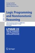
Fig. 1.
The vertex elimination process of an eight-node cycle
×
Example 5
Let G be the cycle depicted in Fig. 1a. Figure 1a to 1g show the vertex elimination process of G according to \(\alpha \), where \(\alpha (1)\) to \(\alpha (8)\) are 2, 4, 6, 8, 1, 5, 3, and 7, respectively. Figure 1h depicts the vertex elimination graph according to \(\alpha \). As it can be seen in Fig. 1, after elimination of each node, the size of the remaining cycle decreases by one node. Therefore, the produced vertex elimination graph must have a cycle of length 2.
5 Translating SAT Modulo Acyclicity into Pure SAT
Let \(\phi \) be a propositional formula associated with graph \(G=\langle {V},{E}\rangle \), such that arc \(\langle {v_i},{v_j}\rangle \,\in \, E\) is represented by the atom \(e_{i,j}\,\in \, \textrm{At}(\phi )\). An interpretation I is an acyclic model of formula \(\phi \) iff \(I\models \phi \) in the classical sense and the digraph \(G_I=(V,\{\langle {v_i},{v_j}\rangle |e_{i,j}\,\in \, I\})\) is acyclic. We are interested in producing a propositional formula \(\phi '\), such that \(\phi '\) is satisfiable in the classical sense if and only if there is an acyclic model for \(\phi \).
Vertex elimination has recently been used for translating SAT modulo acyclicity into pure SAT [21]. This is achieved by adding atoms and clauses to \(\phi \) that dynamically simulate the vertex elimination process of \(G_I\) for a classical model I of \(\phi \). Considering the cycle contraction property of vertex elimination graphs mentioned above, the acyclicity of \(G_I\) can then be ensured by prohibiting cycles of length 2 in the vertex elimination graph of \(G_I\).
Let \(\alpha \) be an arbitrary ordering of V. Without loss of generality, we assume that members of V are indexed such that for \(i=1,\ldots ,n\), \(\alpha (i)=v_i\). For the sake of simplicity, we denote the vertex elimination graphs of G and \(G_I\) according to \(\alpha \), simply by \(G^*=\langle {V},{E^*}\rangle \) and \(G^*_I=\langle {V},{E^*_I}\rangle \), respectively. To simulate the vertex elimination process of \(G_I\), we need atoms \(e'_{i,j}\) to represent the arcs of \(G^*_I\). We know that every arc of \(G_I\) is also an arc of \(G^*_I\). In other words, \(e_{i,j}\) implies \(e'_{i,j}\). Hence, we add to the original formula
Let \(G=G_0, G_{1},\ldots ,G_{n-1}\) be the vertex elimination process of G, and \(G_I=G'_0,G'_{1},\ldots ,G'_{n-1}\) be the vertex elimination process of \(G_I\). Since \(G_I\) is a subgraph of G, \(G'_i\) must be a subgraph of \(G_i\) for \(i=1,\ldots ,n-1\). Therefore, the fill-in of \(v_i\) in \(G'_{i-1}\) is also a subset of the fill-in of \(v_i\) in \(G_{i-1}\). Since the fill-in of \(v_i\) in \(G_{i-1}\) can be computed statically, we can use it to reduce the number of formulas and atoms needed for dynamic computation of the fill-in of \(v_i\) in \(G'_{i-1}\). Based on this, we add formula (12) to ensure that for \(i=1,\ldots ,n-1\), the fill-in of \(v_i\) in \(G'_{i-1}\) is included in \(G^*_I\). In (12), \(F_{i-1}(v_i)\) denotes the fill-in of \(v_i\) in \(G_{i-1}\).
Consider \(\phi '\) to be the conjunction of \(\phi \) and formulas (11) to (13). Theorem 1 and Theorem 2 of [21] show that for any given ordering \(\alpha \) of V, \(\phi '\) is satisfiable in classical sense iff there is an acyclic model for \(\phi \). Nevertheless, by straightforward consideration, one can reach to a stronger theoretical result as follows.
Proposition 4
Let \(\phi \) be a propositional formula subject to acyclicity constraint, associated with graph \(G=\langle {V},{E}\rangle \), and \(\alpha \) be any ordering of V.
1.
If an interpretation \(I\subseteq \textrm{At}(\phi )\) is an acyclic model of \(\phi \), then the interpretation \(J=I\cup \{{e'_{i,j}}\mid {\langle {v_i},{v_j}\rangle \,\in \, E^*_I}\}\) is a classical model of \(\phi '\).
2.
If an interpretation \(J\subseteq \textrm{At}(\phi ')\) is a classical model of \(\phi '\), then the interpretation \(I=J\cap \textrm{At}(\phi )\) is an acyclic model of \(\phi \).
6 Translating ASP into Pure SAT
Considering a WCP P, let \(\phi \) denote the conjunction of all clauses produced by the translation \(\mathrm {Tr_{COMP}}(\mathrm {Tr_{ACYC}}(\mathrm {Tr_{NORM}}(P)))\). By construction, \(\phi \) is a propositional formula with acyclicity constraint imposed on a graph \(G=\langle {V},{E}\rangle \), where V is the set of ordinary (non-dependency) atoms in \(\mathrm {Tr_{NORM}}(P)\), and E is the set of pairs \(\langle {a},{b}\rangle \) such that \(\texttt{dep}(a,b)\) is an atom in \(\mathrm {Tr_{ACYC}}(\mathrm {Tr_{NORM}}(P))\). Let \(G=G_0, G_{1},\ldots ,G_{n-1}\), \(F_{i-1}(v_i)\), and \(G^*=\langle {V},{E^*}\rangle \) be defined as in Sect. 5 and \(\mathrm {Tr_{SAT}}(P)\) the set of clauses in \(\phi \) extended by clauses derived from formulas (11)–(13). Theorem 1 is a direct consequence of Propositions 1–4.
Theorem 1
Let P be a WCP.
1.
If an interpretation \(M\subseteq \textrm{At}(P)\) is a stable model of P, then there is a classical model N of \(\mathrm {Tr_{SAT}}(P)\) such that \(M=N\cap \textrm{At}(P)\).
2.
If an interpretation \(N\subseteq \textrm{At}(\mathrm {Tr_{SAT}}(P))\) is a classical model of \(\mathrm {Tr_{SAT}}(P)\), then \(M=N\cap \textrm{At}(P)\) is a stable model of P.
Theorem 1 does not provide a bijection between the set of classical models of \(\mathrm {Tr_{SAT}}(P)\) and the set of stable modes of P but admits the following result.
Corollary 1
Let P be a WCP. The set of projections of classical models of \(\mathrm {Tr_{SAT}}(P)\) to \(\textrm{At}(P)\) is equal to the set of stable models of P.
Example 6
Consider the clauses of Example 4. After our vertex elimination based translation, clauses \(\lnot \texttt{dep}(a,c)\vee \mathtt {dep'}(a,c)\) and \(\lnot \texttt{dep}(c,a)\vee \mathtt {dep'}(c,a)\) are produced according to formula (11), and \(\mathtt {dep'}(a,c)\vee \lnot \mathtt {dep'}(c,a)\) is produced by formula (13), rendering \(\mathrm {Tr_{SAT}}(P)\) not satisfiable by any superset of N from Example 3. \(\blacksquare \)
7 Experimental Evaluation
We have implemented our vertex elimination based translation of SAT modulo acyclicity into pure SAT as Graph2SAT 1.0 within the ASPTOOLS1 collection [14]. To translate ASP to SAT modulo acyclicity, we use lp2acyc 1.30, lp2normal2 1.14, lp2sat 1.26, all provided by the ASPTOOLS collection. All experiments are run on a cluster of Linux machines with Intel Xeon 2.40 GHz CPUs, using a timeout of 600 s per problem, and, a memory limit of 16 GB. For determining the vertex elimination order, we implemented the minimum degree heuristic. As the SAT solver, we use Kissat 1.0.3 [2].
Table 1.
Comparison of coverage of competing methods
Problem Set
Problems
Solved
SAT
CLASP
WASP
GRAPHSAT
BIN
CombinedConfiguration
99
66
65
19
26
33
Hamiltonian
300
282
199
276
300
194
KnightTourWithHoles
300
44
40
37
31
26
Labyrinth
246
205
209
191
109
156
MazeGeneration
50
50
50
50
50
22
RandomNonTight
14
14
14
12
14
14
Total
1219
661
577
585
530
445
Fig. 2.
Cumulative numbers of problems solved by the competing methods
×
As regards competing methods, we compare against state-of-the-art native ASP solvers Clasp 3.3.5 and Wasp 2.0, the translation-based method using SAT modulo acyclicity formulas fed to Graphsat as the solver, as well as the previously introduced binary counter encoding of acyclicity constraint into pure SAT [13] accompanied by Kissat as the solver, henceforth denoted by Bin. As the benchmark set, we use all problem sets of previous ASP competitions whose complexity is not beyond NP and are in the non-tight decision category. The problem sets with such properties are: CombinedConfiguration, KnightTourWithHoles, Labyrinth, MazeGeneration, and RandomNonTight. We also use the Hamiltonian cycle encoding presented in [19]. This problem set includes 30 randomly generated planar graphs with 60, 70, ..., 150 nodes, summing up to 300 instances. In total, 1219 problem instances are used in our experiments. Here, we report the solving times of the competing methods. The time spent by our method on translation is negligible compared to the solving time. We checked that taking the translation time into account would not render any of the currently solved instances unsolvable within the time limit of 600 s.
Fig. 3.
Cumulative numbers of problems solved by the competing methods in each problem set
×
The number of problems solved by the mentioned methods on our benchmark suite is stated in Table 1. In total, our method solves 84, 76, 131, and 221 problems more than Clasp, Wasp, Graphsat, and Bin, respectively. Figure 2 shows the cumulative number of problems solved by the competing methods. As it can be observed, when given more than 30 s, our method solves more problems than any other competing solver. Also, Fig. 3, which depicts the cumulative number of problems solved by the competing methods in each problem set, shows that our method is among the top two solvers in every problem set.
8 Discussion and Conclusion
In this work, we take into reconsideration the translation of ASP into SAT modulo graphs and, more specifically, SAT modulo acyclicity [8, 9]. This transformation along its refactored version [4] enable the computation of answer sets using appropriately extended SAT solvers such as GraphSAT. The recent approach of [21] makes the graph extension involved in SAT modulo acyclicity obsolete using yet another transformation based on vertex elimination. The central goal of this work is to check the effect on performance if the composition of these translations is deployed and a state-of-the-art SAT solver [2] is used as the back-end solver. The results obtained for six non-tight benchmarks are very promising as the approach presented in this work turns out to be competitive against GraphSAT and the native ASP solvers Clasp and Wasp. This can be interpreted as a realization of the long-term objective of translation-based ASP, i.e., taking advantage of the development of solver technology. An immediate conclusion is that the designs of native ASP solvers should be revised to reflect recent developments in SAT solvers. Otherwise, the performance gap is to grow.
Acknowledgments
Financial support from the Academy of Finland (Project XAILOG, #345633) is gratefully acknowledged.
Open Access This chapter is licensed under the terms of the Creative Commons Attribution 4.0 International License (http://creativecommons.org/licenses/by/4.0/), which permits use, sharing, adaptation, distribution and reproduction in any medium or format, as long as you give appropriate credit to the original author(s) and the source, provide a link to the Creative Commons license and indicate if changes were made.
The images or other third party material in this chapter are included in the chapter's Creative Commons license, unless indicated otherwise in a credit line to the material. If material is not included in the chapter's Creative Commons license and your intended use is not permitted by statutory regulation or exceeds the permitted use, you will need to obtain permission directly from the copyright holder.
 ). Then I satisfies a rule \(r\,\in \, P\) of forms (1) and (3), denoted \(I\models r\), if the satisfaction of the body, denoted \(I\models \textrm{body}(r)\), implies that \(\textrm{head}(r)\,\in \, I\), i.e., \(I\models \textrm{head}(r)\). For a choice rule r of form (2), \(I\models r\) unconditionally. Moreover, the interpretation I is a (classical) model of P if \(I\models r\) holds for every \(r\,\in \, P\). Each positive program P has a unique least model \(\textrm{LM}(P)\) obtained as the intersection \(\bigcap \{{I\subseteq \textrm{At}(P)}\mid {I\models P}\}\).
 . Finally, for an entire WCP P, the reduct \({P}^{I}=\bigcup \{{{r}^{I}}\mid {r\,\in \, P}\}\) and I is a stable model of P iff \(I=\textrm{LM}({P}^{I})\). For the purposes of this work, it is also useful to distinguish the supporting rules of P with respect to I, i.e., \(\textrm{SR}_{P}(I)=\{{r\,\in \, P}\mid {\textrm{head}(r)\,\in \, I, I\models \textrm{body}(r)}\}\). Then, a model \(I\models P\) is supported (by P) when \(I=\{{\textrm{head}(r)}\mid {r\,\in \,\textrm{SR}_{P}(I)}\}\). Each stable model of P is supported by P, but supported models are not necessarily stable, such as \(I=\{a\}\) for \(P=\{a\leftarrow a.\}\).
 . Then, if a defining rule \(r\,\in \,\textrm{def}_{P}(a)\) is of the form (1) or (2), the rule (4) below captures well-support mediated by r, but if it is of the form (3), then the rule is (5).
For the program \(\mathrm {Tr_{ACYC}}(P)\) obtained in this way, the distinction between stable and supported models disappears if we insist on acyclic models I for which the digraph induced by the set of arcs \(\{{\langle {a},{b}\rangle }\mid {\texttt{dep}(a,b)\,\in \, I}\}\) is acyclic.
. Then, if a defining rule \(r\,\in \,\textrm{def}_{P}(a)\) is of the form (1) or (2), the rule (4) below captures well-support mediated by r, but if it is of the form (3), then the rule is (5).
For the program \(\mathrm {Tr_{ACYC}}(P)\) obtained in this way, the distinction between stable and supported models disappears if we insist on acyclic models I for which the digraph induced by the set of arcs \(\{{\langle {a},{b}\rangle }\mid {\texttt{dep}(a,b)\,\in \, I}\}\) is acyclic.