An average Indian farm size is 1.08 ha (Agricultural Census 2015–16), and it has been shrinking over the decades (it was 2.3 ha in 1970–71).
10.1 Background and Introduction
An average Indian farm size is 1.08 ha (Agricultural Census 2015–16), and it has been shrinking over the decades (it was 2.3 ha in 1970–71). India has about 146 million landholdings, and 68.5% of these are marginal holdings, i.e. less than 1 hectare; the average landholding size is much smaller at 0.38 ha. In addition, about 17.7% of Indian landholdings are categorised as small; i.e., they are between 1 and 2 ha and have an average size of 1.41 ha. Thus, about 86% Indian landholdings are less than 2 ha and are called the country’s small and marginal landholdings or farmers (SMF). They together operate on about 47% of the country’s 157 million hectares of operated area.1
As incomes from such small farms would not be enough to sustain families, farmers diversify their sources of income to include livestock like dairy, work as labourers on others’ farms or even outside farms (non-farm), operate small businesses like barber shops, etc. As the landholding size falls, one would expect a more diversified income portfolio. These diversified activities may not all be accounted for as part of the country’s agricultural GDP. While some may be counted towards manufacturing GDP, others may be added to the services sector’s GDP.
Anzeige
We explore this aspect of farmer incomes in detail in this chapter. The focus will be on understanding and analysing:
1.
The level of farmers’ incomes in the country and inequality of incomes between states; and
2.
The structure of farmers’ incomes and trends
The chapter is divided into five sections. In Sect. 10.2, an analysis of farmers’ incomes is presented, with some key highlights. In Sect. 10.3 , the PM’s dream of doubling farmers’ incomes is outlined and key learning from the Dalwai Committee Report is highlighted. In Sect. 10.4 profitability of major crops in important producing states, and major challenges that limit farmers’ incomes are identified, and in the last section, recommendations are made for ways that can support PM Modi’s drive to double/augment farmers’ incomes.
10.2 Analysing Trends and Composition of Farmer Incomes
10.2.1 Estimates of Indian Farmers’ Incomes
An estimate of farmers’ incomes is not a typical macroeconomic aggregate number that is estimated on a regular basis by the Indian government. Instead, it is estimated only occasionally through sample surveys undertaken by the Ministry of Statistics and Programme Implementation (MOSPI) of the Government of India or other government agencies. Since the year 2000, estimates of farmer incomes are available for three years—2002–03, 2012–13 and 2015–16. The 2002–03 and 2012–13 surveys were conducted by the NSSO. The 2015–16 survey was conducted by the National Bank for Agriculture and Rural Development (NABARD) and estimates are available in the NABARD All India Financial Inclusion Survey (NAFIS) report.
There is some difference between the NSSO and NABARD surveys in the definition of “farmer” as well as their coverage, which is explained below in more detail.
Anzeige
For the 2012–13 survey, GoI’s National Sample Survey Office (NSSO) surveyed about 35,200 households2 to profile income sources of an average Indian farmer. It found that an average Indian farmer had four major sources of incomes: (i) income from cultivation (includes income from production of field crops and plantation/orchard crops); (ii) income from livestock (includes receipts from sale of milk, eggs, live animals, wool, fish, honey, hide, bones, manure, etc.); (iii) wages and salaries (includes income from working on others’ farms; it also includes salaries from working in construction sector, wages received under MGNREGA, etc.) and (iv) income from non-farm work (receipts from sale of prepared food, refreshment and drinks, earnings from goods and passenger traffic, communication charges receivable from customers (STD/courier, fax, etc.), receipts for educational activity (like tuition fees, examination fees, capitation fees, etc.)).
NABARD’s NAFIS surveyed about 40,327 households and like the NSSO, estimated sources and levels of farmers’ incomes. On two accounts, however, the estimates of farmers’ incomes from the two surveys are not strictly comparable.
1.
The definition of the “rural” sector: NABARD covers Tier 3 (population between 20,000 and 50,000), Tier 4 (10,000–20,000), Tier 5 (5000–10,000) and Tier 6 (less than 5000) areas whereas NSSO covers only Tier 6 areas.
2.
Type of farmers studied: While NAFIS included households who earned at least Rs. 5000 from agricultural and allied activities in the year; this threshold for the NSSO was Rs. 3000.
Based on these, it may not be inaccurate to say that estimates of farmer income estimates presented by NAFIS are likely to have an upward bias as compared to NSSO’s estimates. This is because (a) it studies areas with larger populations, which are likely to offer better income opportunities; and (b) because of a higher income threshold, NAFIS profiles a relatively richer farmer than one studied under NSSO.
As on October 2020, there is no updated estimate from NSSO after its 2012–13 survey, therefore one is left with little choice for analysis but to use NAFIS results.
Additionally, it may be important to note that all the three years for which we have data on farmers’ income were rain-deficient years. The years 2002–03 and 2015–16 were drought years, i.e., when the actual rainfall fell short of its long-period average (LPA) by more than 10% (the drought threshold for India), while 2012–13, rainfall was −7.1% below LPA. It, therefore, is likely that the available income estimates are lower than what they would be in normal rainfall years. It is also possible that during drought years, when crops fail, farmers are forced to move out and work as labourers outside farming. This may raise the share of wages and salaries in comparison to income coming from the cultivation of crops.
10.2.2 Level and Structure of Farmers’ Incomes
In 2002–03, an average Indian farming household earned about Rs. 2115 per month of which about Rs. 970 was earned from cultivation, Rs. 91 from livestock activities, about Rs. 818 from wages and salaries and Rs. 236 from non-farm business activities.
In 2012–13, the average total income of a farming household increased to Rs. 6427 per month. Of this, Rs. 3081 came from cultivation, Rs. 763 from livestock, Rs. 2071 from wages and salaries and Rs. 512 from non-farm business.
In 2015–16, the total average income of an average farming household went up to Rs. 8931 per month, of which Rs. 3140 came from cultivation, Rs. 711 from livestock, Rs. 4469 from wages and salaries and Rs. 611 from non-farm business.
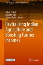
In the 13 years between 2002–03 and 2015–16, these incomes grew at an average CAGR of 11.8%. With the consumer price index for agricultural labourers (CPI-AL) increasing at 8.1%, the CAGR of a farmer’s real income works out to be about 3.7%. Breaking up the farmer incomes into its four components, the sharpest CAGR is observed in the case of incomes coming from livestock as they are estimated to have grown at 17.1% in the 13 years. A summary of an average farming household’s nominal incomes and their composition is presented in Fig. 10.1. Annexure Table 10.1 contains state-wise composition of farming household’s income for the period of 2002–03 to 2015–16.
Two graphs. A bar graph of average farm income in I N R per month for 2002 to 2003, N S S O; 2012 to 2013, N S S O, and 2015 to 2016, N A F I S, is 2115, 6427, and 8931, respectively. A stacked bar graph depicts cultivation, and wages and salaries are the highest share of income for farmers for the years 2002 to 2003 and 2012 to 2013, and 2015-16, respectively.
Fig. 10.1
Average farm income level and composition of farmer’s incomes.
Source NSSO and NAFIS
×
The statistics reveal some interesting facts about the composition of the income of a farmer:
1.
Share of income from cultivation and livestock—The share of income from the two activities has fallen between 2002–03 and 2015–16. From 50% (in 2002–03), it first increased to 60% (in 2012–13) and subsequently fell to 43% (in 2015–16). In actual terms though, income earned from these two activities increased, albeit marginally, throughout the period: from Rs. 1060 (2002–03), to Rs. 3844 (2012–13) to Rs. 3851 (2015–16)
2.
Income from livestock—Barring income from livestock, the absolute level of income did not fall for any other income component in the studied years. Incomes increased from Rs. 91 (share of 4% in the total income) in 2002–03 to Rs. 763 (share of 12% in total income) in 2012–13 but then fell to Rs. 711 (share of 8% in total income) in 2015–16.
3.
Share of income coming from wages and salaries (W&S)—In the three years under the study, the share of income from wages and salaries shows a trend that is opposite to the trend observed in the income from cultivation. By 2012–13, the share of income from cultivation rose (from 46% in 2002–03 to 48%), and that of income from W&S fell (from 39 to 32%). Then by 2015–16, while the share of income from cultivation fell to 35%, but that from W&S increased to 50%.
4.
Income from the non-farm sector—This component of farm incomes is the smallest and has grown the slowest.
These are crucial indicators for policy makers, but the fact that the data (as also mentioned above) were collected in drought years does cast doubts on their usefulness.
In a drought year, reduced activity on the farm will push several small and marginal farmers to work as agricultural labourers on other’s farms to sustain their families. Thus, the falling share of income from cultivation and rising share of W&S observed above is plausible. However, 2015–16 was not just a normal drought year; it was the second consecutive drought year after 2014 (a situation that happened only three times in India’s 100 years of rainfall history before this) and that raises questions about the year being an outlier and the data being representative of an exceptionally vulnerable year, thus making it incomparable with data points in other years.
The fact that NAFIS studied larger and richer areas compared to those studied under the NSSO also makes the 2015–16 data incomparable to the extent that it is likely to have an upward bias in incomes from off-farm activities (including W&S).
Hopefully future surveys, if timed for normal rainfall years and done for individuals with similar profiles, will throw better light on the trends of various components of farming household incomes.
Farmers’ Incomes as per Landholding Sizes
Normally, one expects that with shrinking landholding size, farmers’ incomes will also decline. This is also borne by data from NAFIS for 2015–16.
India’s marginal farmers (i.e., ones operating on less than 1 ha of land) earned between Rs. 6650 and Rs. 8171 per month and small farmers (i.e., those operating on 1–2 ha of land) earned about Rs. 9990 per month. The highest incomes were earned by the larger farmers, i.e. those operating on landholding of greater than 2 ha, who earned about Rs. 14,682 per month.
In terms of sources of incomes vis-à-vis the average landholding size, the share of income from cultivation increases with an increase in the land holding size. Smaller landholder households earned most of their income from livestock and through wages and salaries (see Fig. 10.2).
Two graphs. A bar graph plots hectares versus incomes in I N R per month. Farmers holding greater than 2 hectares earn the highest income of 14682 while the income of all sizes combined is 8931 and it is highlighted. A stacked bar graph depicts farmers with less than .01 hectares and greater than 2 hectares earn high in wages and salaries, and cultivation, respectively.
Fig. 10.2
Landholding-wise incomes (INR/month) and composition of farmers’ incomes by landholding size.
Source Data from NABARD’s NAFIS
×
10.2.3 Farmers’ Income in Indian States
Overall Trends
There is wide variation in the average agricultural household incomes across states. As per NABARD’s NAFIS, the highest incomes (monthly basis) were earned by Punjab farmers (Rs. 23,133 per month), followed by Haryana (Rs. 18,496 per month), Kerala (Rs. 16,927 per month) and Gujarat (Rs. 11,899 per month). Low incomes were earned by farmers in the eastern Indian states of Odisha (Rs. 7731 per month), Bihar (Rs. 7175 per month) and Jharkhand (Rs. 6991 per month) and the southern state of Andhra Pradesh (Rs. 6920 per month); the lowest incomes were earned by UP farmers (Rs. 6668 per month).
A map of India is categorized based on income level. It includes 6000 to 7878, 7 states; 7878 to 8931,3 states; 8931 to 10624, 11 states; 10624 to 23133, 7 states; and all India 8931. All values are in I N R per month. Uttar Pradesh, Bihar, Jharkhand, West Bengal, Odisha, Andhra Pradesh, and Tripura fall under the 6000 to 7878 categories.
Fig. 10.3
Farmers’ average monthly incomes in major Indian states: 2015–16 (INR/month).
Source Created by authors from NAFIS data
Figure 10.3 presents the average monthly farmer income levels in different Indian states. The darker the green colour gets, the higher the average level of income. In states coded in grey, farmers earn low levels of income. As can be seen from the map, these states are Uttar Pradesh, Bihar, Jharkhand, West Bengal, Odisha and Andhra Pradesh, and, as per Census 2011, these states are home to close to 40% of Indian farmers.
Mapping Cultivators and Farmers’ Incomes
As per Census 2011, India has a total agricultural workforce of about 263 million of which around 119 million are cultivators (i.e. who own land or have the right to operate land) and the remaining, i.e. about 144 million work as agricultural labourers (i.e. who do not own land and work on farms owned by others in return for wages paid to them in cash or kind). We mapped state-level farmers’ incomes (2015–16 as per NABARD’s NAFIS) with the states to which the cultivators belonged and found two interesting trends (Fig. 10.4).
A graph of I N R per month and percent share in total India cultivators versus 28 states of India. The decreasing bars indicate the share of Indian cultivators. Uttar Pradesh is the highest with 16 %. The fluctuating line indicates farmer's average income. Punjab is the highest with 23000. Another line indicates all-India farmer's average income, which is constant at 8000. All values are estimated.
Fig. 10.4
Mapping cultivators with farmers’ incomes.
Source NABARD’s NAFIS and Census 2011
1.
States that were home to about 50% of Indian cultivators (UP, Rajasthan, Maharashtra, Madhya Pradesh and Bihar) earned the lowest in the country. In India, UP has the largest number of cultivators (16% of India’s cultivators), and this state has the lowest level of farmers’ incomes.
2.
Less than 5% of Indian farmers earned the highest incomes in the country: Punjab, Haryana and Kerala together account for 4.3% of Indian cultivators, and their average monthly income is about Rs. 19,519,3 which is more than twice the Indian average.
×
It is to be noted that income levels are low for a majority of cultivators. States mentioned in (1) above must be focal states for any strategic action by the Indian government to enhance farmer incomes in the country. Their abysmally low current levels of incomes offer an opportunity, much like a low-hanging fruit, to double their incomes quickly. This was proven by the eastern Indian state of Odisha as shown below.
Growth Rates of Farmers’ Incomes Across Major States
Although farmers in eastern states like Bihar, Odisha and West Bengal earn very low levels of income compared to the more successful northern states of Punjab, Haryana or the western state of Gujarat, income growth rates can be pretty high. This is clearly demonstrated by Odisha, where farmers’ real incomes increased by CAGR of 8.4% between 2002–03 and 2015–16. UP (3.9%), Bihar (3.7%) and Andhra Pradesh (3.5%) hovered very close to the all-India trend rate of 3.7%. In J&K, real farm incomes fell between 2002–03 and 2015–16 (Fig. 10.5).
A line graph of growth rate for 2002-03 to 2015-16 for India and its 19 states. Odisha spots the highest with 8.4 and Jammu and Kashmir spots the lowest with negative 2.3.
Fig. 10.5
Growth in farmers’ real incomes (CAGR), 2002–03 to 2015–16.
Source NSSO & NABARD
×
Composition of Farmers’ Income
According to NSSO estimates from the “Situation Assessment Survey”, an increasing share of agricultural household income has been from cultivation with its contribution growing from 45.8% in 2002–03 to 47.9% in 2012–13. Government policy documents (Dalwai Committee Report), based on the results of the NSSO survey, have targeted raising the share of income from cultivation and livestock to 70% by 2022–23. However, an analysis of the composition of farmers’ income based on NAFIS data shows that a major share of income came from wages in 2015–16 (50% of total income). Wage employment as a vital source of livelihood in rural India is not surprising. It is widely experienced that as an economy grows, the labour force gradually shifts from farm to non-farm activities.
State-wise analysis shows that in most states, the share of income from wages in 2015–16 was higher than at the national level; among them, Jammu and Kashmir (71%), Tamil Nadu (69.8%), Bihar (66.3%), Rajasthan (63.2%), Uttarakhand (57.2%) and Odisha (56.5%) are states where the wage income is high. In the period from 2002–03 to 2015–16, the scale of increase in the contribution of wages to total income is the highest for Uttarakhand (41.2% points) followed by Bihar (38.8% points) and Jammu & Kashmir. Punjab and Karnataka are the only two states that experienced a marginal decline (1% point) in the contribution of income coming from wages. Temporal changes in the composition of income are presented in Table 10.1.
In the NSSO survey, non-farm business is defined as all household economic activities other than those covered under farm business. It included manufacturing, mining and quarrying, trade, hotels and restaurants, transport, construction, repairing and other services. The share of income coming from “non-farm businesses” decreased from 11.2% in 2002–03 to 8% in 2012–13 and further to 6.8% in 2015–16. Among the states, Assam (24.7%) has the highest share of income coming from non-farm businesses, followed by West Bengal (18.1%) and Odisha (9.6%) (Fig. 10.6).
A stacked bar graph exhibits the composition of income, in percentage, for net receipts from non-farm business, wages, and cultivation and farming of animals and a decreasing line graph indicates the growth rate for 2002-03 to 2015-16. The bar for India is annotated.
Fig. 10.6
State-wise farmers’ income growth (2002–03 to 2015–16) and composition of farmers’ income, 2015–16.
Source NSSO and NABARD
×
The analysis also reveals that except for Bihar, Jammu and Kashmir and West Bengal, there has been an increase in the share of income coming from rearing and farming of animals between 2002–03 and 2012–13 in all states. A significant increase in the share is observed for Rajasthan (32% point), Haryana (29% point) and Madhya Pradesh (22.7% points) with more than a 20% point increase in the share of income coming from cultivation and farming of animals.
From 2012–13 to 2015–16, the data shows a major decline in the share of income coming from cultivation and farming of animals except in Kerala. States like Assam, Bihar, Jammu & Kashmir and Uttarakhand show a more than 20% point decline in the share of income coming from cultivation and farming of animals, and this decline is compensated by a huge increase in the share of income from wages. Such a major change in the structure of income in the period of three years seems unlikely, and this may well be the result of the use of different definitions and samples in the two surveys.
×
10.2.4 Agricultural GDP Growth and Farmer Incomes
Higher returns on cultivation encourage farmers to invest more, which raises agricultural GDP, which in turn augments farmers’ income. However, higher agricultural GDP growth rates, interestingly, may or may not result in higher growth in incomes of farming households. Among the six states presented in Fig. 10.7, despite high AGDP growth, farmer incomes have failed to rise as fast in Gujarat and MP (to some extent). Contrarily, farmers’ incomes have risen sharply in Odisha, Punjab, UP and Bihar despite the not-so-impressive AGDP performance.
A pair of bar graphs of G S D P A and farmer income C A G R for India, Bihar, Gujarat, Madhya Pradesh, Odisha, Punjab, and Uttar Pradesh, for the year 2002-03 and 2015-16. The values are as follows, (3.4, 3.7), (1.9, 3.7), (6.3, 4.2), (7.3, 6.6), (3.7, 8.4), (1.7, 4.3), and (2.4, 3.9), respectively. All values are in percentage.
Fig. 10.7
CAGR of GSDPA and FY between 2002–03 and 2015–16.
Source MOSPI, NSSO and NABARD. Note: Growth rates are estimated as CAGR of terminal values of Agricultural and allied-GDP and farmers’ income for the years 2002–03 and 2015–16
×
Some parts of this disconnect between AGDP, and farm income trends may be explained by the way the data for each are segregated and analysed. Certain sources of incomes like wages and salaries that agricultural HHs made from, for example, working in schools, tuition centres, etc., will be counted as income from services and not attributed to agriculture; hence, even though an agricultural HH earned that income, it does not get reflected in agricultural GDP. Similarly, although income from fisheries will be accounted for in GDP from agriculture and allied activities, it will not be counted in data on farmers’ incomes. This and many more data issues raise the need to look at both agricultural GDP and the level of farmer incomes to monitor their impact on poverty alleviation in the country.
Major Findings
After analysing farmers’ incomes, a few striking trends become apparent4:
1.
The share of income coming from cultivation has been falling: In 2002–03, 46% of monthly farmers’ incomes came from cultivation, and by 2015–16, this share has fallen to 35%.
2.
The share of income from livestock has grown from 4% (2002–03) to 8% (2015–16). However, the trend reverses when one looks at the data between 2012–13 and 2015–16—both the absolute level and share in total income from livestock has fallen.
3.
Wages and salaries are the most important source of incomes for Indian farmers (2015–16). In a country with shrinking landholdings, farmers inevitably rely on jobs in the informal and formal sector. Experience around the developing world, especially in China, has revealed that in a booming economy, normally it is the construction sector that absorbs much of the labour force coming out of agriculture. In India, the government offers employment guarantee programmes like MGNREGA, which could have absorbed some agricultural labour, especially during drought years. However, this outmigration from agriculture to non-farm activities requires a much more detailed study, which is not attempted here. However, one upshot is clear: for the first time, in the years mentioned above, farm families seem to have derived more than half their income from wages and salaries.
4.
Trends in farmers’ incomes may or may not necessarily follow the agricultural GDP growth path of a state.
10.3 PM’s Dream to Double Farmers’ Incomes
The Prime Minister of India, Shri Narendra Modi, made a call to double farmers’ incomes by 2022 at a kisan (farmer) rally in Bareilly on 28 February 2016. It was not clear initially whether it was a political statement expressing his “dream” or an announcement of a policy measure followed by a strategic plan of action. However, the statement assumed a serious note when Finance Minister Arun Jaitley mentioned this in his budget speeches of 2016–17 and 2017–18. It was followed by the setting up of a committee for doubling farmers’ income (DFI) in April 2016 under the chairmanship of Ashok Dalwai. The Committee submitted its final report [referred to hereafter as the Dalwai Committee Report (DCR)] to the GoI in September 2018.
What does doubling of farmers’ incomes mean?
As per the DCR, the PM’s target was to double the real incomes of farmers in seven years, i.e. by 2022–23 over the 2015–16 income level. In 2015–16, DCR estimated, by extrapolating 2012–13 survey data, that farmers’ average income was about Rs. 8059 per month (as per NABARD’s NAFIS, the 2015–16 estimate of farmers’ income was Rs. 8931). The DCR also makes it clear that the target of doubling farmers’ incomes by 2022–23 was in real terms, not nominal. That would amount to raising their 2015–16 levels of income to Rs. 16,118 per month (in real terms) in seven years, i.e. by 2022–23 (as per NAFIS’s estimate, the target 2022–23 income level would be Rs. 17,862) (Fig. 10.8).
Two bar graphs. Farmer's income in I N R per month is on the left. The highest bar is for N A F I S, 2022-23 with 17862. 2 bars on the right, is for the years 2002-03 and 2015-16, and 2015-16 and 2022-23. The values are 3.7 and 10.4, respectively.
Fig. 10.8
What doubling income means: actual and required CAGR (%).
Source DCR, NSSO and NAFIS
×
Between 2002–03 and 2015–16, average income of farmers grew in real terms at a CAGR of 3.7%. To achieve the DFI target, the required growth rate at the all-India level was estimated to be 10.4%, i.e. 2.8 times the growth rate achieved historically.
To achieve this, DCR prepared 14 volumes (containing close to 3000 pages) proposing strategies on almost every aspect of agriculture. This voluminous report has summarised recommendations in Volume 14 that presents about 619 recommendations. Some of these are highlighted below.
Improvement in Crop Productivity:
Given the inelastic nature of land and high concentration of farmers’ families, achieving high productivity is crucial for food security as well as global competitiveness. The report proposes increasing the per hectare productivity of millets from 1.1 to 1.6 tonnes, pulses from 0.7 to 1.4 tonnes and oilseeds from 0.96 to 1.5 tonnes, respectively. It also suggested a shift from the current measurement of grain per hectare approach to a grains (in calories) plus nutrients/ha approach. Location-specific causes of the yield gap need to be identified, and strategies should be outlined to close that gap.
Improvement in Livestock Productivity:
To augment farmers’ incomes through livestock, the productivity of dairy animals has to be increased. Steps like quality artificial insemination, genome selection and embryo transfer for sustainable breed improvement and incentivising feed mills to produce compound feed should be the major areas of intervention. The report suggests dissemination of region-specific technologies to cultivate green fodder in uncultivable, saline land. Scarcity of quality fodder should be dealt with through development of hybrids of fodder crops, perennial grasses, legumes, etc. Silage making of surplus green fodder can be helpful in the lean season.
Resource-use efficiency:
The report points out that moving from food security to income security for farmers requires diversification of the system from crop to high value products. Diversification in turn promotes resource-use efficiency. The recommendations include making the soil health card scheme more practical and flexible; bringing in more technical competence in collecting and testing soil samples; encouraging private sector infrastructure and so on. According to the report, soil health-related issues can be dealt with by linking the soil health card portal with the integrated fertiliser management system (I-FMS); facilitating soil testing at reasonable cost, preparing district-level nutrient maps and other steps like organic farming, adopting an ecosystem-based approach to plant nutrition etc.
The Dalwai committee accepted the fact that earlier policies to achieve food security did not consider sustainability issues and that cost us water security. Water-related recommendations include testing and recording water health on the lines of the soil health card, recycling wastewater and encouraging micro-irrigation. Since there is no single law dealing with groundwater legislation across the country, the reports talk about implementing the proposals made in the model bill drafted by the CGWB.
Efficient Monetisation of Farm Produce:
DCR extended the concept of the post-production value chain by going beyond agricultural marketing to “monetisation”. According to this, the objective should be to obtain the best possible value for farm produce by facilitating the efficient transfer of produce from farms to the end-consumer. Major recommendations include the development of well-functioning warehouse facilities, promotion of warehouse-based post-harvest loans, special focus on building aggregation units at the village level for horticulture produce and developing marketing co-operatives. To establish a more efficient market model, it has proposed a new structure comprising primary rural agricultural markets (PRAM), competitive wholesale markets and export markets. This is proposed keeping in mind that small and marginal farmers dominate the agricultural space in India, but they fail to reap benefits of marketing infrastructure and hence do not receive the right price for their produce. The committee proposes that PRAM could be used as an aggregation platform. The recommendations also include adopting the Model Agriculture Produce and Livestock Marketing (APLM) Act, 2017, and increasing the number of wholesale and retail markets to 10,000 and 20,000 respectively.
Given that farm families are engaged in agriculture for about 185 days a year, the Dalwai committee recommended the creation of additional productive jobs, utilising primary products and by-products of farming activities using local skills. These secondary incomes could help farmers in times of volatility and falling prices. The report recommends that these activities be promoted by exempting these activities from GST or keeping tax rates low, providing special category funding and incentivising micro-enterprises led by women.
The committee has produced a comprehensive and detailed analysis of the current agricultural situation in India. The committee has estimated the additional investments needed to attain an annual growth rate in farmers’ income of 10.4% growth at about Rs. 640,000 crore at 2011–12 prices, of which the government’s contribution would be 80%. It also targets raising the share of monthly income of farmers coming from cultivation and livestock from the present level of 60% (in 2012–13 survey) to 70%5 (in one place it says even 80%)6 over the target period (2016–17 to 2022–23).
While the efforts of Dalwai Committee are well appreciated and the government has instituted a mechanism to track the implementation of recommendations, four major questions remain unanswered:
(i)
Under the business as usual scenario based on, say, the last 10–15 years, growth rates of agricultural GSDP and in farmers’ incomes have been around 3.6% (page: 25, Report of the Committee on Doubling Farmers’ Income Volume II “Status of Farmers’ Income: Strategies for Accelerated Growth”). Is it feasible to set a double-digit target at the national level for doubling farmers’ income in the coming years until 2022–23?
(ii)
Where will the government mobilise the additional fund of Rs. 6.4 lakh crore at 2011–12 prices that is mentioned in the report, especially when loan waivers and other welfare schemes are on the rise?
(iii)
Even if the government succeeds in mobilising funds for the extra investment and it does achieve the 10.4% growth in farmers’ incomes, who will absorb the massive surpluses in agricultural production? What is the rate at which domestic consumption of agricultural goods has been rising over the last 10–15 years? What is the growth in agricultural exports? In fact, during the period from 2014–15 to 2018–19, exports of agricultural products have come down compared to where they were in 2013–14. Given this, does the economy have the capacity to absorb such a high growth rate in agriculture and farmers’ incomes?
(iv)
How, in such a short period, is the government going to implement the interventions listed in the report?
The key issue with these reports is that there are way too many recommendations in it and by the time the final DCR Report; i.e. Volume 14 titled “comprehensive policy recommendations” was released, two and a half years of the total seven-year period envisaged by PM Modi to double farmers’ real incomes had already elapsed.
During the five-year tenure of the Modi government, i.e., 2014–15 to 2018–19, the average annual agricultural GDP growth rate of the country was 2.9%. If one assumes that farmers’ incomes broadly increase in line with the rate of growth of agricultural GDP, as has been the case in the last decade, it is obvious that the country lags far behind the required CAGR of 10.4%, the annual growth rate required to achieve PM Modi’s dream of doubling farmers’ real incomes by 2022–23. This means that in the remaining years until 2022–23, farmers’ real incomes need to increase by about 13–15% per annum. This appears almost impossible with the set of policies followed during the last five years.
If the country has to reach anywhere near the goal of doubling the real incomes of farmers by 2022–23, it cannot be done without increasing the profitability of cultivation and livestock farming. In the next section, we look at the historical trends in the profitability of major crops and identify the factors influencing profitability.
10.4 Profitability in Major Crops in Important Producing States
In this section, we look at the net profitability of major crops produced in India. We concentrate on two variants of the cost of cultivation. A2 is the paid out costs by the farmer and includes the value of hired labour and machinery, value of owned machine labour, value of seeds, fertilisers, manure, pesticides, irrigation charges, land revenue, interest on capital and rent paid on leased in land. C2 includes paid out costs by farmers plus imputed rental costs of owned land, imputed interest on owned capital and imputed value of family labour employed. Since the BJP election manifesto of 2014 had promised implementing the Swaminathan Committee formula for pricing, which suggested a 50% profit over C2 cost, our analysis involves estimating profitability over both A2 and C2 costs. Profitability is calculated by subtracting A2 and C2 costs per hectare from the gross value of output per hectare. Data on the actual value of output and cost per hectare are available up to 2015–16. Major producing states are considered for our analysis. Profitability at the all-India level is calculated by taking the weighted average of net profits of the states, the weights being the share under a particular crop in the total GCA under that crop in a state. The results show that the net profit margin differs across states as well as crops, but in most cases, margins have fallen in the period from 2012–13 to 2015–16, the latest years for which actual cost of cultivation is available. We briefly discuss these below. The figures showing profitability over C2 cost are presented in the annexure.
Paddy
Rice is the most widely produced and consumed crop in India. The top five paddy producing states are West Bengal, Uttar Pradesh, Punjab, Andhra Pradesh and Tamil Nadu. Other important producers are Bihar and Odisha. These states together account for 59% of the area under paddy cultivation and contribute 63% of the total production. The results indicate that, barring Punjab, profits have declined in all states (there was a marginal fall in profitability in the years 2014–15 to 2015–16 in Punjab too). Profitability based on C2 cost has turned negative in some states (West Bengal, Odisha and Uttar Pradesh). In 2015–16, Punjab farmers had a 203% margin over A2 cost. This is not surprising given that farmers in Punjab receive assured minimum support price, which at least covers their cost. Farmers in most other rice producing states, barring Andhra, generally do not get even MSP for paddy. The weighted average of these seven states shows the net margins over A2 cost falling from 108% in 2013–14 to 90% in 2015–16 (Fig. 10.9) while the net margin over C2 cost has fallen from 8% to minus 4% in the same period (Fig. 10.23).
A grouped bar graph exhibits the profit margin as a % of A 2 cost for Paddy in West Bengal, Uttar Pradesh, Punjab, Andhra Pradesh, Tamil Nadu, Bihar, Odisha, and major states, weighted average, over 4 years from 2012-13 to 2015-16. Punjab spots high in all 4 years.
Fig. 10.9
Profit margin as per cent of A2 cost for paddy.
Source Calculated by the authors using DES cost of cultivation data
×
Wheat
Wheat is another important staple consumed all over India. The crop is mostly cultivated in the temperate region of western India in the rabi season. Uttar Pradesh, Madhya Pradesh, Punjab, Haryana and Rajasthan are the largest producers of wheat accounting for 80% of the GCA under the crop and 86% of total wheat production. Comparatively, wheat farmers appear to be better placed than paddy farmers. All the top producing states have a positive margin over A2 cost. But unfortunately profit margins have declined for all major states. At the all-India level, (calculated by taking the weighted average based on share in GCA), the profit margin over A2 cost and C2 cost has declined from 183 and 35%, respectively in 2012–13 to 155 and 19.5%, respectively, in 2015–16 (Figs. 10.10 and 10.24).
A grouped bar graph exhibits the profit margin as a % of A 2 cost for wheat in Uttar Pradesh, Madhya Pradesh, Punjab, Haryana, Rajasthan, and major states, weighted average, over 4 years from 2012-13 to 2015-16. Rajasthan spots high in 2012-13, 2013-14, and 2015-16.
Fig. 10.10
Profit margins as a percentage of A2 cost for wheat.
Source Calculated by authors using DES cost of cultivation data
×
States like Punjab, Haryana and MP have a well-functioning procurement mechanism. Punjab procures 74% of rice and 67% of the wheat produced in the state while Madhya Pradesh procures 53% of its total wheat production. The Madhya Pradesh government launched a bonus policy over and above the centre’s MSP, which has helped increase production and procurement of wheat in the state (Gulati et al. 2017). But in states like Bihar, Odisha and UP, the procurement mechanism is poor and the farm harvest price remained consistently lower than the announced MSPs.
Maize
After rice and wheat, maize is the most widely produced cereal in India and is used as both food and fodder. Maize is a kharif crop, but in some states, it is also cultivated during the rabi season. Our analysis shows that maize is unprofitable in all the major producing states (Figs. 10.11 and 10.25). Even though Punjab, Haryana and western Uttar Pradesh have geographical conditions that are suitable for maize cultivation, they continue growing rice and wheat due to the latter’s higher profitability that is largely facilitated by a robust procurement mechanism under the MSP regime. The profit margin in the case of maize over A2 and C2 cost declined from 101% and 18%, respectively, in 2012–13 to 79% and −3%, respectively, in 2015–16.
A grouped bar graph of the profit margin as a % of A 2 cost for Maize in Karnataka, Bihar, Madhya Pradesh, Tamil Nadu, and major states, weighted average, over 4 years, from 2012-13 to 2015-16. Madhya Pradesh is high in 2012-13 while Bihar spot high from 2013-14 to 2015-16.
Fig. 10.11
Profit margins as per cent of A2 cost for maize.
Source Calculated by authors using DES cost of Cultivation Data
×
Arhar
India is the largest producer, consumer and importer of pulses in the world. It is considered a cheap source of protein for the poor. Pigeon pea is an important item in the consumption basket of the Indian population. Madhya Pradesh, Maharashtra, Gujarat, Karnataka and UP are the largest producing states, together contributing 76% of the total production of arhar(also called tur) in India. Pulse prices have experienced major volatility in the past few years as did net profitability (Figs. 10.12 and 10.26 ). Due to severe back-to-back droughts during 2014–15 and 2015–16, the production of all pulses plummeted to 16.5 MMT. Increased imports by India put pressure on international prices. The price of tur dal in the retail market shot up to Rs. 180 per kg and the farmers responded to this price signal by bringing more area under pulses, and a good rainfall led to a bumper harvest in 2016–17. Tur production, for example, shot up by a massive 65%, from 2.5 MMT to 4.2 MMT, while overall, pulses production went up by 33% from 16.5 MMT to 22 MMT. This resulted in a substantial drop in the market price of tur, from about Rs. 10,000/quintal in September–October 2016 to Rs. 4000–4500/quintal in February–March 2017, even below the MSP. Such low prices did not bring much profit compared to other crops. This was evident in the 2016–17 profitability figures.
A bar graph of the profit margin as a % of A 2 cost for Arhar in Madhya Pradesh, Maharashtra, Gujarat, Karnataka, U P, and major states, weighted average over 4 years. Madhya Pradesh is high in 2012-13 and U P spot high from 2013-14 to 2015-16.
Fig. 10.12
Profit margins as per cent of A2 cost for Arhar.
Source Calculated by authors using DES cost of Cultivation Data
×
Sugarcane
Sugarcane is one of the major cash crops produced in India and the crop consumes a lot of water. The largest producers include Uttar Pradesh, Maharashtra, Karnataka and Tamil Nadu, which together produce 80% of the total production. In both UP and Maharashtra, sugarcane is cultivated in irrigated areas. Sugarcane is a 9-month crop in UP, which need to be irrigated 7–8 times. As against this, in Maharashtra, it needs to be irrigated at least 25 times. In terms of profit margins, sugarcane cultivation is more profitable in Uttar Pradesh than in Maharashtra and other significant producing states. However, all states including Uttar Pradesh have experienced a reduction in profit margins between 2012–13 and 2015–16 (Figs. 10.13 and 10.27).
A grouped bar graph of the profit margin as a % of A 2 cost for sugarcane plots for 4 states and a weighted average over 4 years. U P and Karnataka spot high in various years.
Fig. 10.13
Profit margin as per cent of A2 cost for sugarcane.
Source Calculated by authors using DES cost of cultivation data
×
The sugar sector has also been facing the same kind of volatility faced by pulses in recent years. Domestic sugar production dropped to 20.3 MMT, which led to an increase in demand for imports and domestic ex-mill sugar prices crossed Rs. 36 per kg. As a result, farmers expanded the area under sugarcane and a good monsoon led to an improvement in the yield and recovery ratio. The production of sugar increased from 20.3 MMT in 2016–17 to 32.3 MMT in 2017–18. This helped reduce imports but during these time, world prices of sugar dropped by 50%. It made Indian sugar non-competitive in global markets.
Cotton
Cotton is the most important fibre crop produced in India. The significant producers include Gujarat, Maharashtra, Andhra Pradesh, Karnataka and Telengana that together account for 82% of the total production. After the introduction of BT cotton in India, production increased enormously. The export of raw cotton increased from $10 million in 2002–03 to $4258 million by 2011–12. But, international prices crashed thereafter and the value of export started declining and eventually reached $1536 million by 2016–17. Consequently, the net profit margin on cotton across states has declined. The weighted average margin of major producing states shows a steady decline, especially in the last two years (Figs. 10.14 and 10.28).
A grouped bar graph of the profit margin as a % of A 2 cost for cotton plots for 4 states and a weighted average over 4 years. Karnataka is high in 2012-13. Maharashtra is high in 2013-14. Gujarat is high in 2014-15 and 2015-16.
Fig. 10.14
Profit margin as a percentage of A2 cost for cotton.
Source Calculated by authors using DES cost of cultivation data
×
Soybean
Soybean is the most important form of edible oil consumed in India. Among all the food groups consumed in India, consumption of edible oil has been increasing at the highest pace. Domestic production is insufficient to fulfil growing demand, and India is heavily import dependant. Of the total soybean produced in the country, more than 90% is contributed by Madhya Pradesh, Maharashtra and Rajasthan. There has been a steep decline in net profit in the last three years (Figs. 10.15 and 10.29).
A grouped bar graph of the profit margin as a % of A 2 cost for Soyabean plots for 3 states and a weighted average over 4 years. Rajasthan is high in 2012-13 and 2015-16. Madhya Pradesh is high in 2013-14 and 2014-15.
Fig. 10.15
Profit margin as a percentage of A2 cost for soybean.
Source Calculated by authors using DES cost of cultivation data
×
Onion
Onion is one of the most important commercially grown vegetables, and India is the world’s second largest producer with production of 21 million MT in 2015–16. The largest producers of onions include Maharashtra, Karnataka, Madhya Pradesh, Bihar and Gujarat. Unfortunately, we only have profitability data for the states of Maharashtra, Karnataka and Gujarat that together contribute 52% of total production. Onions are always in the news for the volatility in its prices and consequently in its profit margin (Figs. 10.16 and 10.30). One of the major reasons behind high volatility in onion prices is the lack of storage facilities that have not kept pace with rising production. Our analysis shows that all the states experienced volatility in the profit margin in the past four years (Fig. 10.16). This boom and bust in onion prices takes place almost every alternate year. In 2017 (May–June), onion prices went down to around Rs. 2/kg in various mandis in Madhya Pradesh. This resulted in a farmers’ agitation, police firing and unfortunate deaths. The immediate band-aid measure was procuring onions at Rs. 800/quintal; due to the scarcity of storage facilities, 8.76 lakh tonnes of onion was disposed of through the public distribution system (PDS) at almost one-fifth the cost. Since then, onion prices have moved up and down several times. Major investment needs to be made to improve the cold chain infrastructure and processing facilities.
A grouped bar graph of the profit margin as a % of A 2 cost for onion plots for 3 states and a weighted average over 4 years. Karnataka scored high in 2012-13, 2013-14, and 2015-16. Gujarat scored high in 2014-15.
Fig. 10.16
Profit margin as percentage of A2 cost for onion.
Source Calculated by authors using DES cost of cultivation data
×
To summarise the crop-wise results, the profitability of important crops in major producing states has actually declined over the four years covered. We have calculated the weighted average profitability of major crops from state-level profitability by using the share of the state in the total cropped area under that crop. The unfortunate truth is that the net profit margin in almost all major agricultural commodities covered here has declined in recent years. Farmers cultivating paddy, maize, sugarcane, cotton and soybean all experienced losses in 2015–16 compared to previous years (Figs. 10.17 and 10.18).
A grouped bar graph of the profit margin as a % of A 2 cost for 13 different grains over 4 years. Onion spots high in 2012-13. R and M spots high in 2013-14, and 2014-15. Arhar spots high in 2015-16.
Fig. 10.17
Trends in profitability (over A2 cost) of important crops in India (weighted average of major producing states).
Source Calculated by the authors using DES cost of cultivation data
A positive-negative grouped bar graph of the profit margin as a % of C 2 cost for 13 different grains over 4 years. Onion spots high in 2012-13. Sugarcane spots high in 2013-14. Potato spots low in 2014-15. Soybean spots low in 2015-16.
Fig. 10.18
Trends in profitability (over C2 cost) of important crops in India (weighted average of major producing states).
Source Calculated by the authors using DES cost of cultivation data
×
×
It may be noted that there is normally a lag of two to three years to get data on the cost of cultivation from government sources. But in recent years, some major kharif crops were in the news because of the high volatility in their prices. Hence, it would be interesting to see the recent trends in profitability of major kharif crops (kharif seasons of 2016, 2017 and 2018). Actual market prices have been obtained by taking the weighted average of market prices in the major markets of the largest producing states, the weights being the share of the state in the total production of that crop. As state-wise actual cost figures are not available for the period of analysis, the projected cost derived by CACP for calculating MSPs is taken as a proxy.
Figures 10.19 and 10.20 show that farmers producing kharif crops are incurring huge losses, particularly so in kharif 2017. In 2018, profit margins recovered in the case of some crops but not enough to compensate for the decline in 2017. No wonder, one witnessed a large number of farmers’ agitations during 2018, just ahead of the 2019 parliamentary elections.
A double bar graph of the margin with market price over A 2 cost for 8 grains over 3 years. Cotton is high in 2016. Paddy is high in 2017. Arhar is high in 2018.
Fig. 10.19
Net margin (market price-projected A2 cost) as percentage of projected A2 cost.
Source Agmark.net, CACP
A grouped positive-negative bar graph of the margin with market price over projected C 2 cost as a % of C 2 cost for 8 grains over 3 Kharif years. Cotton is high in Kharif 2016. Urad is low in Kharif 2018. Moong is the lowest in Kharif 2017.
Fig. 10.20
Net margin (market price-projected C2 cost) as percentage of projected C2 cost.
Source Agmark.net, CACP
×
×
If margins over costs were not improving, and in fact falling over the last five to seven years, the absolute profits on a per hectare basis could still have improved if productivity gained sufficiently to compensate for the losses in profit margins. However, productivity growth in most crops has also remained sluggish during the last 15 years or so, suggesting that real profits even on a per hectare basis may have been shrinking. The productivity of major crops has increased very slowly over the years (Fig. 10.21 and Table 10.2). Compared to neighbouring countries, India’s productivity gain is very poor. In 2016–17, paddy (rice) and wheat productivity in China stood at 6.9 MT/ha and 5.4 MT/ha, respectively (FAOSTAT). In the same year, India’s productivity was 3.8 MT/ha and 2.7 MT/ha for rice and wheat, respectively. Productivity of rice in India is even lower than in Bangladesh. Given the inelastic nature of land, increasing population and the need to ensure global competitiveness, stagnant productivity can affect profitability more severely unless prices rise sufficiently.
A line graph of the productivity of sugarcane from 2000-01 to 2016-17 plots superimposed lines for sugarcane, wheat, maize, rice, groundnuts, R and M, Soybean, Arhar, Urad, cotton, and moong.
Fig. 10.21
Productivity of important crops in India.
Source Directorate of Economics and Statistics
×
Rising production costs have also affected profitability. Figure 10.22 shows that in the period of 2004–05 to 2015–16, there was a steady increase in production costs (in 2011–12 prices) for all major crops. The cost of production of maize, arhar, urad, groundnuts and onion increases at an annual rate of more than 8% in real terms while the increase was more than roughly 5% in the case of the rest of the crops. This is a cause for concern as it reflects that productivity gains, whatever little there has been, have not reduced real costs of production on a per unit basis. And if output prices too have not risen sufficiently in line with rising costs, the inevitable result is shrinking margins. Historical crop wise cost of production and year on year growth rate of A2 cost of production is tabulated in the annexure Tables 10.3 and 10.4.
A line graph of the real, A 2, cost of production from 2004-05 to 2015-16. It plots superimposed lines for onion, potato, sugarcane, groundnuts, cotton, paddy, arhar, wheat, maize, soybean, R and M, urad, and moong.
Fig. 10.22
Cost (A2) of production (Rs/ha) of major crops, 2004–05 to 2015–16.
Source Directorate of Economics and Statistics
×
Rising costs and tumbling margins do not auger well for doubling farmers’ incomes by 2022–23 as envisaged by the PM. These trends need urgent attention; otherwise, falling incentives in cultivation will also adversely impact capital formation in agriculture by farmers, further slowing down the growth rate of agricultural GDP, which has already fallen from 4.3% during UPA-2 (2009–10 to 2013–14) to just 2.9% during Modi period-1 (2014–15 to 2018–19).
With such slow growth, it emerges nearly impossible for the governmnet to be able to double incomes of farmers by year 2022–23. But there are countries, like China, which managed to achieve this miracle in the early years of reform. China increased its farmers’ real incomes by almost 15% per annum during 1978–84 just by focusing on land reforms (dismantling the commune system and adopting the household responsibility model) and substantially freeing prices from government controls. There are still a wide range of opportunities available that can help boost Indian farmers’ incomes, if not double them, by 2022. The issue of markets and low prices is a current problem, given that imports have flooded the markets and exports have not increased in the last five years. Market reforms, along with strategic changes in trade policy, are low-hanging fruits and need to be initiated immediately. They will improve market price realisation for farmers. Substantial improvements in productivity by carrying out supply side reforms (agricultural R&D, irrigation, fertilisers, power, etc.) can cut down costs and improve margins for farmers. The business as usual (BAU) scenario cannot double farmers’ incomes in the absence of any major reform of agricultural markets or of measures to step up productivity substantially.
Dairy
Livestock constituted 29.3% of the value of output from agriculture and allied activities while milk alone contributed 14% of GVOA in 2015–16. However, of total income, only 8% was contributed by the livestock sector in the same year. India has experienced unprecedented growth in milk production since 2014–15. Currently, India is the largest producer of milk in the world, and it provides livelihood to small and landless agricultural households. However, in 2017–18 milk prices declined by 20–30% in major milk producing states creating a stress in the dairy industry. Farmers in those states protested by spilling milk on the streets. The situation of over production was worsened by plummeting global skimmed milk powder (SMP) prices from around $4744/tonne in 2013–14 to $1925/tonne in 2017–18. As a result, India’s SMP exports declined from 124 thousand tonnes in 2013–14 to 11.3 thousand tonnes in 2017–18, adversely affecting farmers’ profitability and incomes. There is no market price assurance for countless small farmers struggling to manage their livelihood by selling liquid milk. India needs to create demand to match increasing supplies of milk by investing in value added products. The government can introduce milk in mid-day meal schemes to boost demand.
10.5 Challenges in Augmenting Incomes
Apart from the constraints highlighted in the section above, the following challenges make it difficult to augment farmer incomes.
1.
Shrinking land and landholding size—resource-use efficiency is adversely affected by land constraints.
2.
Productivity as a route to higher production—As highlighted in previous chapters, yields for several crops and in many states have been stagnating or falling. This may be due to the use of inappropriate seeds, inefficient use of fertilisers, inability to adjust and adapt to changing weather and climatic conditions, etc.
3.
Inadequate access to credit—As per NABARD’s NAFIS, between July 2015 and June 2016, 43.5% agricultural HHs took loans. Of these, 60.5% took institutional loans and about 9% took loans from both institutional and non-institutional sources. This means that about 30.3% Indian agricultural HHs took loans from institutions, implying that about 70% of agricultural HHs took loans from non-institutional (NI) sources, which includes borrowing from relatives, friends, moneylenders, landlords, input suppliers, etc. Anecdotal evidence suggest that the interest charged on NI loans was anywhere between 2 and 3% per month. This lack of access to credit adversely affects a farmer’s ability to invest.
4.
Highly volatile crop prices—Volatility in crop prices arise because:
i.
There is dearth of storage facilities and an individual farmer is too small and poor to invest in storage facilities on his farm.
ii.
Processing facilities and value chains do not exist, leading to a price slump during a bumper crop year. This is typically the case with most horticultural crops.
iii.
Insufficient markets—As per Dalwai Committee Report (Volume 4, pp 57), Indian farmers on average have to travel about 12 km to access a market and this distance varies between states. In Assam, this distance is about 45 km, while it is only 6 km in Punjab. As per the National Commission on Agriculture (1970), the ideal distance should be 5 km.
5.
Inadequate access to relevant techniques and production technology.
6.
Low cropping intensity due to lack of access to water.
Challenges for income from livestock
1.
Dairy: Here the biggest challenges are threefold: breed of the animal (and thus its genetic yields), feed for the animal and inadequate demand for the final product, i.e. milk. The high costs of artificial insemination and inadequate availability of high-yielding cattle/buffalo semen forces dairy farmers to rear inefficient animals. Besides, the increasing cost of feed, shrinking grasslands for open grazing due to the growing pressure on land, inadequate knowledge of the appropriate balanced diet for animals, and lack of access to vaccination facilities for animals reduce yields further. Central to all these problems in the lack of formal milk processing centres in the country, the absence of which causes prices to fluctuate widely.
10.6 Conclusion
It is apparent from the analysis that the relentless focus of government(s) on increasing agricultural GDP may not by itself increase farmers’ incomes and thus farmers’ welfare. Despite achieving high agricultural GDP growth rates, farmers’ incomes in states like Gujarat and Madhya Pradesh did not grow as fast. In contrast, there were states like Odisha, Bihar and, to some extent, UP where despite average agricultural GDP growth rates, farmers’ incomes grew rapidly.
Overall, PM Modi’s dream of doubling the 2015–16 level of farmer incomes by 2022–23 is unlikely to be realised, mainly on two accounts—(a) four of the seven years have gone by with an average agricultural GDP growth rate of 3.7% (much lower than the required rate of 10.4%); and (b) the profitability of cultivation has been declining due to plummeting agricultural prices in recent years and rising cultivation costs, mainly on account of rising labour costs.
Nevertheless, the drive to enhance farmers’ incomes should continue. Interventions required to achieve this at the policy and operational level are discussed and presented in the next chapter.
Open Access This chapter is licensed under the terms of the Creative Commons Attribution 4.0 International License (http://creativecommons.org/licenses/by/4.0/), which permits use, sharing, adaptation, distribution and reproduction in any medium or format, as long as you give appropriate credit to the original author(s) and the source, provide a link to the Creative Commons licence and indicate if changes were made.
The images or other third party material in this chapter are included in the chapter’s Creative Commons licence, unless indicated otherwise in a credit line to the material. If material is not included in the chapter’s Creative Commons licence and your intended use is not permitted by statutory regulation or exceeds the permitted use, you will need to obtain permission directly from the copyright holder.
A grouped positive-negative bar graph of the Profit Margin as a share of C 2 cost in percentage for Paddy for 7 states and major states over 4 years. Punjab spots high in all years.
Fig. 10.23
Profit margin as percentage of C2 cost for paddy.
Source Calculated by the authors using DES cost of cultivation data
A grouped positive-negative bar graph of the profit margin as a share of C 2 cost in percentage for Wheat for 5 states and major states over 4 years. Rajasthan scored high in 2012-13, and 2013-14. Uttar Pradesh scored low in 2014-15. Punjab scored high in 2015-16.
Fig. 10.24
Profit margin as percentage of C2 cost for wheat.
Source Calculated by the authors using DES cost of cultivation data
A grouped positive-negative bar graph of the profit margin as a share of C 2 cost for Maize for 4 states and Major states over 4 years. Bihar spots high in 2012-13, and 2013-14. Karnataka and Madhya Pradesh scored low in 2014-15, and 2015-16, respectively.
Fig. 10.25
Profit margin as percentage of C2 cost for maize.
Source Calculated by the authors using DES cost of cultivation data
A grouped positive-negative bar graph of the profit margin as a share of C 2 cost for Arhar for 5 states and Major states over 4 years. Madhya Pradesh spots high in 2012-13 and 2013-14. Karnataka spots high in 2014-15. Gujarat spots high in 2015-16.
Fig. 10.26
Profit margin as percentage of C2 cost for arhar.
Source Calculated by the authors using DES cost of cultivation data
A grouped bar graph of the net margin as a share of C 2 cost for sugarcane for 4 states and major states over 4 years. Karnataka scored high in 2012-13. U P scored high in 2013-14, 2014-15, and 2015-16.
Fig. 10.27
Profit margin as percentage of C2 cost for sugarcane.
Source Calculated by the authors using DES cost of cultivation data
A grouped positive-negative bar graph of the net margin as a share of C 2 cost for cotton for 4 states and major states over 4 years. Andhra Pradesh spots low in all years.
Fig. 10.28
Profit margin as percentage of C2 cost for cotton.
Source Calculated by the authors using DES cost of cultivation data
A grouped positive-negative bar graph of the profit margin as a share of C 2 cost for soybean for 3 states and Major states over 4 years. Rajasthan is high in 2012-13. Maharashtra is high in 2013-14 and low in 2014-15. Madhya Pradesh is low in 2015-16.
Fig. 10.29
Profit margin as percentage of C2 cost for soybean.
Source Calculated by the authors using DES cost of cultivation data
A grouped positive-negative bar graph of the profit margin as a % of C 2 cost for onion for 3 states and Major states over 4 years. Karnataka spots high in 2012-13, 2013-14, and 2015-16, and low in 2014-15.
Fig. 10.30
Profit margin as percentage of C2 cost for onion.
Source Calculated by the authors using DES cost of cultivation data
Table 10.1
Composition of agricultural households’ income (percent of total monthly income), 2002–03 to 2015–16
Major states
Net receipt from cultivation and farming of animals
Net receipts from non-farm business
Income from wages
2002–03
2012–13
2015–16
2002–03
2012–13
2015–16
2002–03
2012–13
2015–16
Andhra Pradesh
51.2
51.8
40.3
9.5
6.7
7.7
39.4
41.5
52.0
Assam
61.2
74.8
25.7
8.1
3.8
24.7
30.8
21.4
49.6
Bihar
61.4
56.1
29.4
11.2
6.7
4.3
27.5
37.2
66.3
Gujarat
60.3
61.4
53.6
5.2
4.8
6.0
34.5
33.9
40.3
Haryana
43.7
72.8
50.2
12.4
3.0
2.0
44.0
24.2
47.8
Himachal Pradesh
36.4
44.7
39.8
16.4
9.4
3.7
47.3
45.9
56.5
Jammu & Kashmir
51.2
30.5
27.1
11.3
11.7
1.9
37.5
57.8
71.0
Karnataka
53.4
62.6
54.3
6.4
7.1
6.5
40.2
30.3
39.2
Kerala
31.8
34.5
46.2
17.9
21.3
1.0
50.3
44.2
52.8
Madhya Pradesh
53.8
76.5
53.8
7.1
2.1
2.5
39.2
21.5
43.8
Maharashtra
57.1
59.5
48.3
10.4
11.3
9.4
32.4
29.2
42.4
Orissa
33.1
54.7
34.0
12.9
10.8
9.6
54.0
34.5
56.5
Punjab
61.7
69.3
63.1
8.9
4.2
8.4
29.5
26.5
28.5
Rajasthan
24.3
55.9
34.9
13.6
9.7
1.9
62.1
34.5
63.2
Tamil Nadu
37.1
43.2
25.1
9.6
15.2
5.1
53.3
41.6
69.8
Uttar Pradesh
54.4
69.0
40.1
11.3
7.6
4.3
34.2
23.4
55.6
West Bengal
39.2
30.3
32.2
18.2
16.3
18.1
42.7
53.4
49.7
Jharkhand
45.3
56.0
44.2
10.0
5.0
3.6
44.7
39.0
52.2
Chhattisgarh
49.9
64.3
40.6
6.2
0.0
4.1
43.8
35.7
55.2
Uttarakhand
68.7
71.9
34.3
15.4
5.4
8.4
16.0
22.7
57.2
India
50.1
59.8
43.1
11.2
8.0
6.8
38.7
32.2
50.0
Table 10.2
Productivity of major crops (MT/ha)
Rice
Wheat
Maize
Arhar
Moong
Urad
Sugarcane
Cotton
Soybean
Groundnuts
R&M
2000–01
1.9
2.7
1.8
0.62
0.32
0.35
68.6
0.19
0.82
0.98
0.94
2001–02
2.1
2.8
2.0
0.68
0.34
0.41
67.4
0.19
0.94
1.13
1.00
2002–03
1.7
2.6
1.7
0.65
0.26
0.38
63.6
0.19
0.76
0.69
0.85
2003–04
2.1
2.7
2.0
0.67
0.50
0.43
59.4
0.31
1.19
1.36
1.16
2004–05
2.0
2.6
1.9
0.67
0.29
0.38
64.8
0.32
0.91
1.02
1.04
2005–06
2.1
2.6
1.9
0.76
0.28
0.39
66.9
0.36
1.07
1.19
1.12
2006–07
2.1
2.7
1.9
0.65
0.33
0.41
69.0
0.42
1.06
0.87
1.10
2007–08
2.2
2.8
2.3
0.83
0.41
0.48
68.9
0.47
1.23
1.46
1.00
2008–09
2.2
2.9
2.4
0.67
0.35
0.42
64.6
0.40
1.04
1.16
1.14
2009–10
2.1
2.8
2.0
0.71
0.18
0.36
70.0
0.40
1.02
0.99
1.18
2010–11
2.2
3.0
2.5
0.66
0.54
0.56
70.1
0.50
1.33
1.41
1.19
2011–12
2.4
3.2
2.5
0.66
0.47
0.52
71.7
0.49
1.21
1.32
1.12
2012–13
2.5
3.1
2.6
0.78
0.44
0.63
68.3
0.49
1.35
0.81
1.26
2013–14
2.4
3.1
2.7
0.81
0.47
0.55
70.5
0.51
1.01
1.73
1.19
2014–15
2.4
2.7
2.6
0.73
0.50
0.60
71.5
0.46
0.95
1.48
1.08
2015–16
2.4
3.0
2.6
0.65
0.42
0.54
70.7
0.41
0.74
1.40
1.18
2016–17
2.5
3.2
2.7
0.91
0.50
0.63
69.0
0.51
1.18
1.32
1.30
Source Agricultural Statistics at a Glance. Various Issues
Table 10.3
Cost of production of major crops in 2011–12 prices (Rs/ha)
Paddy
Wheat
Maize
Arhar
Moong
Urad
Sugarcane
Cotton
Soybean
Groundnuts
R&M
Onion
Potato
2004–05
17,084
16,390
8513
10,426
5268
5976
33,338
21,727
12,405
16,888
9486
31,494
43,879
2005–06
17,759
16,763
11,542
11,460
6698
6545
41,792
22,038
11,611
16,742
10,053
35,782
47,502
2006–07
17,251
17,021
10,675
11,471
7219
7406
41,800
21,705
13,046
15,897
9857
31,633
51,587
2007–08
17,441
16,837
12,459
12,190
6838
7872
40,774
22,449
12,615
18,292
9975
39,149
52,811
2008–09
19,702
17,735
13,676
13,002
6453
7408
38,736
25,955
13,790
21,421
10,345
40,994
42,757
2009–10
21,669
18,600
14,372
12,617
6977
9771
42,633
25,832
15,202
21,598
10,251
34,843
58,420
2010–11
21,894
18,350
15,047
18,145
9288
10,628
50,190
28,568
13,993
24,572
9233
41,556
49,709
2011–12
22,471
19,129
15,645
16,312
9883
9434
54,307
32,452
13,906
29,218
11,317
43,115
42,153
2012–13
23,021
19,835
16,428
19,927
10,887
10,780
54,675
34,155
17,176
31,828
13,009
43,515
47,998
2013–14
23,808
20,303
17,793
19,296
9849
10,962
51,928
35,636
17,217
31,724
13,260
46,888
51,533
2014–15
26,601
20,461
18,587
19,394
8602
9385
58,725
36,739
20,344
32,921
13,358
61,125
68,994
2015–16
29,251
23,281
21,106
24,352
10,055
12,218
62,295
38,984
19,932
39,482
15,556
66,530
63,258
Source Cost of Cultivation Data, DES
Table 10.4
Year on year growth rate of real A2 cost of production
As per Agricultural Census 2015–16, operated area includes both cultivated and uncultivated area, provided part of it is put to agricultural production during the reference period. This is different from the net sown area, which refers to the actual acreage under crops in that year, and gross cropped area, which includes the double cropped area.
Because of the difference in the definition of a “farmer” between NSSO and NABARD, as mentioned in the main text, there is a perceptible upward bias in NABARD’s estimates and we use extreme caution in comparing the data between the two surveys.
Page: 150, Chapter 7, Policy Recommendations, Report of the Committee on Doubling Farmers’ Income Volume II “Status of Farmers’ Income: Strategies for Accelerated Growth”.