This chapter introduces the basic types of bonds and considers their valuation. Bonds are an important source of funding for corporations. And even government bonds are relevant to companies, since the yield on government bonds serves as the risk-free rate discussed in Chap. 4. We explain the drivers of bond yields and the term structure of interest rates. Subsequently, we discuss the liquidity and credit risk of corporate bonds, including the role of ratings.
Social and environmental factors are increasingly being integrated in the valuation of corporate bonds. Studying the company’s business model is important for sustainability integration in the credit risk analysis of bonds. This chapter shows how to include a company’s adaptability to sustainability transitions into the credit risk analysis. Companies that can better adapt their business model face a lower credit risk and hence a lower cost of debt. In addition, there is innovation in the form of sustainability-linked bonds, green bonds, and social bonds to cater for sustainable investment projects.
Overview
This chapter introduces the basic types of bonds and considers their valuation. The pricing of bonds is relevant for corporate finance for several reasons. First, the yield on government bonds serves as the risk-free rate discussed in Chap. 4. Second, companies issue bonds to finance their operations. In particular, long-term investments are financed by bonds and equity (see Chaps. 9 and 10 on equity). A key element of this chapter is the analysis of credit risk on corporate bonds. Bond markets are bigger than stock markets, with institutional investors typically holding more bonds than equity. In the case of insurers and pension funds, the main reason for these large bond holdings is to hedge the interest rate risk on their long-term liabilities.
Social and environmental factors are increasingly being integrated in the valuation of corporate bonds. Studying the company’s business model is important for sustainability integration in the credit risk analysis of bonds. This chapter shows how to include a company’s adaptability to sustainability transitions into the credit risk analysis. Companies that can better adapt their business model face a lower credit risk and hence a lower cost of debt. By contrast, companies with limited capability to adapt encounter increased credit risk and a higher cost of debt.
Anzeige
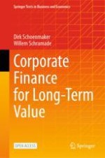
There is innovation in the form of green bonds and social bonds to cater for sustainable investment projects. The challenge is to ‘certify’ the use of the proceeds for green or social projects and to overcome bureaucratic procedures. Yet another type are sustainability-linked bonds, where the interest rate on the bond is directly ‘linked’ to the overall sustainability performance of a company. See Fig. 8.1 for a chapter overview.
4 blocks are labeled sustainable unaware, E S G integrated or inward view, impact or outward view, and integrated value. They have the circles labeled F V, E, and S leading to F V, E V and S V, and F V + E V + S V= I V respectively. They also list a few chapters in each block.
Fig. 8.1
Chapter overview
×
Learning Objectives
After you have studied this chapter, you should be able to:
Explain the basics of bond pricing and valuation
Differentiate between government and corporate bonds
Demonstrate how social and environmental factors can be integrated into bond valuation
Explain that bond investors are more focused on downside protection
Identify the green bond market as an interesting and fast-growing innovation
8.1 Bond Types and Pricing
While equity markets may get more attention, bond markets are actually bigger. At the end of 2020, the value of outstanding government and corporate bonds globally was estimated at $123 trillion (i.e. about 145 per cent of global GDP) versus $112 trillion for outstanding equity (SIFMA, 2021). Bonds come in many forms. They can be complex and varied, but they have a lot in common as well. Bonds are certificates of debt issued by a government, a company, or a financial institution that promise payment of the borrowed amount plus interest by a specified future date.
The biggest bond issuer is the US government. Outstanding US Treasuries amounted to $21 trillion at the end of 2020. Corporate bonds are more dispersed. The largest single corporate bond issuance is a $49 billion corporate bond issued by Verizon Communications to finance its $130 billion acquisition of Vodafone's 45% stake in Verizon Wireless in 2013.
Anzeige
Bond Payments
A bond certificate indicates the amounts and dates of all payments to be made. Payments are made until the final repayment date, known as the maturity date of the bond. The time until the maturity date is known as the term. Bond maturities or terms range from very short term (months) to decades or even perpetuity. There are still some bonds outstanding that were issued centuries ago. Two types of payments are made on a bond:
1.
The promised interest payments, which are called coupons. The bond certificate specifies that the coupons are paid periodically, for example once or twice per year.
2.
The principal or face value of the bond. This is the amount to be paid at maturity. The face value is typically denominated in standard increments such as €1000.
For example, a bond with a face value of €1000 and a 3% coupon (payable annually) will make coupon payments of €30 every 12 months: €1000 * 0.03 = €30. Some bonds do not pay coupon payments. Such bonds are known as zero-coupon bonds and can still offer the same return as coupon paying bonds, by offering the same principal at a lower price.
Types of Bonds
Whereas bonds are public debt, bank loans and private debt placements are types of private debt. Figure 8.2 classifies bonds by the identity of the issuer, with the main distinction being between government and corporate bonds as the latter carry more serious default risk.
A block diagram classifies debts into bonds of public debt and private debt. The bonds are further classified into government bonds and corporate bonds. Corporate bonds are further classified into secured corporate bonds and unsecured corporate bonds.
Fig. 8.2
Classification of bonds
×
Government or sovereign bonds are issued by national governments (i.e. countries). The main distinctions within corporate bonds are those between company issuers and financial sector issuers and between secured and unsecured bonds. The financial sector accounts for a very large part of the corporate bond market (see Table 8.1). In the remainder of this chapter, we focus on government bonds and corporate bonds issued by companies.
Table 8.1
Size of equity and bond markets (end 2020)
Type of securities
Outstanding (in trillions of USD)
Equity markets
112.1
• Public equity
105.8
• Private equity
6.3
Bond markets
123.4
• Government bonds
62.8
• Corporate bonds
60.6
– Issued by companies
17.0
– Issued by financial institutions
43.6
Sources: SIFMA (2021); McKinsey (2022); BIS debt securities statistics
Secured bonds entail specific assets that are pledged as collateral and to which bondholders have a direct claim in the event of bankruptcy. An example is mortgage bonds, which are bonds secured by a pool of mortgages on real estate. Unsecured bonds have lower seniority or priority. In the event of bankruptcy, holders of unsecured bonds have a claim only to the assets of the company that are not already pledged as collateral on other (secured) debt.
Bond Valuation and Its Drivers
In principle, bond prices result from discounting a clear pattern of promised cash flows. The price or value of a coupon bond P equals the present value of all its coupons plus the present value of the face value of the bond with maturity N. The formula is as follows:
where YTMn is the yield to maturity of a zero-coupon bond (a bond without coupons) that matures at the same time as the n-th coupon payment; CPN is the coupon payment; and FV is the bond’s face value, which is typically denominated in standard increments of €1000 or $1000. Bond prices and yields are inversely related. It follows from Eq. (8.1) that a lower yield produces a higher bond price and vice versa. Given that one knows the coupon and face value of a bond, one needs only the price (the yield) to calculate the yield (the price). Below we give examples of both: calculating the yield to maturity (Example 8.1) and calculating the price (Example 8.2). These examples show that once you know one (the yield or the price), you can calculate the other one (the price or the yield).
The coupon payment is determined by the annual coupon rate ACR and the number of coupon payments per year Nr:
$$ CPN=\frac{ACR\ast FV}{Nr} $$
(8.2)
A €1000 bond with a 5% coupon rate and annual payments pays a coupon of €50 = 5% * €1000/1 every year. A €1000 bond with a 6% coupon rate and semi-annual payments pays a coupon of €30 = 6% * €1000/2 every 6 months.
The coupon payments form a stream of equal cash flows paid at regular intervals. In Chap. 4, we call this an annuity (see Eq. 4.7). The present value of the bond then becomes the sum of the ‘coupon annuity’ and the face value. The rates (yields) at which the cash flows need to be discounted do vary, as interest rates fluctuate over time. The yield to maturity (YTM) or just the yield (y) on a bond is the discount rate that sets the present value of its payments equal to its current market price. More formally, the price of a bond P is:
where y is the yield of this particular bond and reflects the yield received if all coupons received are reinvested at a constant interest rate. Put another way, the yield is the IRR (internal rate of return) of a bond. Market forces keep this relation intact: as interest rates and bond yields rise, bond prices fall, and vice versa. This means that bonds trade at times at a premium (at a price greater than face value), at times at a discount (at a price lower than face value), and very occasionally at par (at a price equal to face value).
Example 8.1: Calculating the Yield to Maturity of a Bond
Problem
Consider a 6-year €1000 bond with a 5% coupon rate and annual coupons. If this bond is currently trading for a price of €950.83, what is the bond’s yield to maturity?
Solution
Using Eq. (8.3), we can calculate the yield to maturity:
We can solve it by trial and error. As the price is lower than the face value, the yield to maturity is higher than the annual coupon rate. The yield to maturity appears to be 6%.
Example 8.2: Calculating a Bond Price from Its Yield to Maturity
Problem
Consider a 6-year €1000 bond with a 5% coupon rate and annual coupons. If the yield to maturity is 6%, what is the bond price?
Calculating the price is easier: filling in the formula produces a bond price of €950.83. Of course, this is the same bond price as in Example 8.1. We used the same bond for both calculations.
The price of a zero-coupon bond can be calculated more easily: it is just the present value of the face value:
$$ P=\frac{FV}{{\left(1+{YTM}_n\right)}^n} $$
(8.4)
The yield to maturity YTMn on a zero-coupon government bond is the per-period rate of return for holding the bond from today until maturity n. The zero-coupon yield can be used to calculate the risk-free rate with maturity n. By taking different maturities n = 1, 2, 3, . . , N, we can build the yield curve of N years (see Sect. 8.2 below).
Interest Rate Changes
As stated, interest rates fluctuate and bond prices move along with them. Equation (8.3) shows that if the yield y increases by 1% the effect is larger for a long-term bond than for a short-term bond. This can easily be seen by comparing Eq. (8.3) with N = 1 to that with N = 2 . So longer-term bonds are more exposed to interest rate fluctuations. It is possible to derive an exposure measure to interest rate/yield fluctuations, which is called duration. The duration of a bond is the sensitivity of a bond’s price to changes in interest rates. Duration is the weighted average of the time-length of the cash payments. The time-length is the number of future years n = 1, 2, 3, . . , extending to the final maturity date N. The weight for each year is the present value of the cash flow in that year PV(CFn) divided by the total present value PV of the bond.
The duration is higher for bonds of longer maturity, since more of their cash flows are further in the future, and thus more affected by discount rates. Table 8.2 calculates the duration of 6-year bonds with an annual coupon of 5% and a yield of 4%. The present value PV of the cash flows of each year add up to the total present value PV of €1057.7. Then we calculate the PV of each year’s cash flow as a fraction of total value and multiply each fraction by the year in which that cash flow takes place. The outcomes (see bottom line of Table 8.2) add up to a duration of 5.3 years. As the final payment is relatively large (coupon + face value) and counts heavily (multiplied by year in which discounted), a bond’s duration is close to the bond’s maturity. In Table 8.2, the duration of 5.3 years is close to the bond’s maturity of 6 years. The duration is a good measure of the interest rate risk of a bond. A higher duration (‘weighted maturity’) reflects higher interest rate risk.
Table 8.2
Calculating the duration of 5% 6-year bonds, with a yield to maturity of 4%
Time
2022
2023
2024
2025
2026
2027
Year
1
2
3
4
5
6
Cash flow
€50
€50
€50
€50
€50
€1050
Discount factor
0.962
0.925
0.889
0.855
0.822
0.790
PV(CFn) at 4%
€48.1
€46.2
€44.4
€42.7
€41.1
€829.8
Total PV =
€1057.7
Fraction of total value
0.045
0.044
0.042
0.040
0.039
0.785
Total=
1.0
Year * fraction of total value
0.045
0.087
0.126
0.162
0.194
4.708
Total duration=
5.3
8.2 Term Structure of Interest Rates
Interest rates differ not only over time, they also differ across maturities. This variation is referred to as the term structure of interest rates (also called yield curve): the array of yields on bonds with different terms to maturity. Let’s start with deriving the yield curve from bond prices. To derive a 10-year yield curve, we need to obtain the 1, 2, …, 10-year yield to maturity YTMn. Zero-coupon bonds can be used to find these yields. As Eq. (8.4) demonstrates:
$$ P=\frac{FV}{{\left(1+{YTM}_n\right)}^n} $$
The price of a 1-year zero-coupon bond P gives the 1-year zero-coupon yield YTM1 and so on. Figure 8.3 provides the German yield curve.
A line graph of percentage yield from the German government bonds against residual maturity from 0 to 30 years. It plots a logarithmically increasing curve that increases steeply till 2 years, then increases gradually till 15 years, and then decreases gradually.
Fig. 8.3
German government bond yield curve. Source: World Government Bonds
×
The law of one price can be used to calculate the yields on coupon bonds (with the same liquidity and credit risk). This ‘law’ says that similar products should sell at the same price (see Box 4.1 in Chap. 4). And if they don’t sell at similar prices, the arbitrage mechanism usually makes sure that such differences disappear quickly. Example 8.3 shows how we can calculate the yields on bonds with the same maturity, once we have the yield curve (modelled on the zero-coupon yields). The yield on a coupon bond is basically some sort of weighted average of the cash flows in each period. As the final cash flow (repayment of the face value) dominates, the yield of the 4-year coupon bonds at 4.85% for the 6% coupon bond, and 4.90% for the 4% coupon bond is quite close to the 4-year zero-coupon yield of 5.0% in Example 8.3.
Example 8.3: Law of One Price: Yields on Bonds with the Same Maturity
Problem
Given the following zero-coupon yields, compare the yield to maturity and price of a 4-year bond with 4%, 6%, and zero annual coupons. We use risk-free government bonds.
The bond price calculation is straight-forward. For the yield, we use trial and error. It is interesting to see that the yields on the coupon bonds are just below the yields on zero-coupon bond at 5%. The higher the coupons, the larger the deviation (0.15% for the 6% coupon bond and 0.10% for the 4% coupon bond), since the coupons get a higher weight in the calculation of the yield as weighted average.
Example 8.4: Law of One Price: Yields on Bonds with Different Maturity
Problem
Given the following zero-coupon yields, compare the yield to maturity and price of a 2-year, 3-year, and 4-year bond with a 6% annual coupon. We use risk-free government bonds.
Maturity
1 year
2 years
3 years
4 years
Zero-coupon yield
2.0%
3.0%
4.0%
5.0%
Solution
We can again calculate the bond prices using Eq. (8.1) and the yields using Eq. (8.3). The payoff scheme is provided in the table.
Year (n)
Bond price (P)
Yield (y)
Maturity
1
2
3
4
Zero-coupon yield
2%
3%
4%
5%
Discount factor
0.98
0.94
0.89
0.82
Bond D (6% coupon)
Payment
€60
€1060
PV(CFn)
€58.82
€999.15
€1057.98
2.97%
Bond E (6% coupon)
Payment
€60
€60
€1060
PV(CFn)
€58.82
€56.56
€942.34
€1057.72
3.92%
Bond F (6% coupon)
Payment
€60
€60
€60
€1060
PV(CFn)
€58.82
€56.56
€53.34
€872.06
€1040.78
4.85%
Again, the yields on the coupon bonds are close to the zero-coupon yield with the same maturity. The 2-year bond yield is 2.97% (compared to the 3% zero-coupon yield), the 3-year bond yield is 3.92% (compared to the 4% zero-coupon yield), and the 4-year bond yield is 4.85% (compared to the 5% zero-coupon yield).
In a similar way as in Example 8.3, we can calculate the yields on bonds with different maturities. Example 8.4 shows again that the yield on coupon bonds is quite close to the respective zero-coupon yield with the same maturity. The attentive reader has spotted that Bond B in Example 8.3 is the same as Bond F in Example 8.4. That is an interesting feature of the law of one price. You can make different calculations of bond prices and yields, and you end up with identical prices and yields for ‘similar’ bonds.
Explaining the Term Structure
As bonds with a higher duration are more exposed to interest rate risk, they carry a higher risk premium (or term premium). The yield curve is therefore typically upward sloping. The term premium leads to a positive term spread, i.e. the spread of yields for bonds with longer maturity over yields for bonds with shorter maturity, even when markets expect increasing and decreasing interest rates to be equally likely.
There are several explanations for a positive term premium:
1.
Belief that short-term rates will be higher in the future
2.
Higher exposure of longer-term bonds to changes in interest rates
3.
Risk of higher inflation in the future
So, the first two reasons for a positive term spread concern (the risk of) higher future interest rates. The third reason is about risk-averse investors demanding a premium for inflation risk. Inflation \( {i}_{i,t}=\frac{\left(\ {CPI}_{i,t}-{CPI}_{i,t-1}\ \right)}{CPI_{i,t-1}} \) is the realised consumer price index (CPI) inflation rate in a given country i and year t. Inflation can and does differ across time and across countries. It is therefore helpful to compare yields or more generally returns in real terms rr. The real rate of return can be calculated as:
$$ 1+{r}_r=\frac{1+r}{1+i} $$
(8.6)
By re-arranging, we can express the Inflation-adjusted real returns rr for an asset class as:
We can use the approximation for real interest rates in the form of nominal return minus inflation r − i in low inflation countries. If the nominal rate is 4% and inflation is 1%, the real rate of return is approximately 3 % ≈ 4 % − 1%. The exact real interest rate is 2.97%. For high inflation countries, we’d better use the full formula, since larger numbers result in larger deviations.
Notwithstanding these forces for a positive term premium, a downward sloping yield curve (called inverse yield curve) is also possible. A major reason for an inverse yield curve is increased expectations of a recession, where central banks are likely to reduce interest rates to foster economic growth.
8.3 Government Bonds and Corporate Bonds
This section reviews the main drivers of yields on government and corporate bonds. Next, we calculate the credit risk (also called the risk of default) and the liquidity risk on bonds.
Drivers of Yields on Government Bonds
National government bonds, also known as sovereign bonds, have been issued for centuries and their prices have tended to be driven by (expectations regarding) the fortunes of the states involved and their reliability in paying back their debt. In fact, Ferguson (2001) argues that Britain beat France in the struggle for colonial empire in the 1700s, as the British managed to finance their wars at low interest rates, thanks to reliability in repaying debt and an efficient bureaucracy. France’s cost of funding was consistently higher due to its poor reputation in repaying debt.
Nowadays, countries have formal credit ratings, set by credit rating agencies (as explained in Sect. 8.3 below). In an empirical study of the determinants of sovereign credit ratings, Cantor and Pecker (1996) find that credit ratings and sovereign borrowing costs can be explained by per capita income, GDP growth, inflation, external debt, the level of economic development, and default history. Government bonds are typically bought by institutional investors, who seek a relatively safe investment. Insurance companies and pension funds have large holdings of government bonds to hedge the interest rate risk of their liabilities with safe assets. Government bonds by the same issuer (or by an issuer with the same rating) may still have different prices, driven by differences in maturity and liquidity.
Different dynamics may occur during economic crises, with a prominent role for financial contagion (Beirne & Fratzscher, 2013). Financial contagion is the spread of market disturbances from one market or country to other markets or countries. A salient example is the European Sovereign Debt Crisis, which started in Greece at the end of 2009. After several revisions of previously announced deficit figures (even going back to the time of admission of Greece into the Euro area) had been published it became clear that public finances in Greece were unsustainable. On 10 May 2010, the 10-year yield spread between Greek and German government bonds reached about 10% (outside the range of Fig. 8.4). Similar concerns arose in Ireland, Portugal, and, later, Spain and Italy. Figure 8.4 shows that the Italian 10-yield spread went up to 5% in late 2011 (7% for Italy minus 2% for Germany). Again, the Italian yield spread reached 3% in 2018/2019, due to concerns about political stability in Italy.
A line graph of in percent versus January 08 to January 22 plots 4 fluctuating lines for Germany, France, Netherlands, and Italy. The line for Italy is above all other lines. The time between January 10 and January 13 is shaded.
Fig. 8.4
Ten-year government bond spreads against German government bonds, 2008–2022 (in percent). Source: Bloomberg
×
The European Sovereign Debt Crisis reconfirmed the status of the German bond as benchmark bond. The German bond yield can thus be used as the risk-free rate for the Euro (see Chap. 13). The yield curves of two other very creditworthy countries, France and the Netherlands, are just above the German yield curve in Fig. 8.4. Similarly, the US Treasury yield serves as the risk-free rate for the US dollar. US government bonds are called Treasuries. These German and US government bonds are the most creditworthy and liquid bonds in their respective currencies.
Drivers of Yields on Corporate Bonds
Corporate bonds differ from sovereign bonds in some important respects. The most important differences are that corporate bonds tend to carry more serious default and liquidity risks. Liquidity risk refers to the lower trading frequencies, higher transaction costs due to lower competition among bond traders, and smaller sizes of corporate bonds, which make it harder to trade such bonds. Given that corporates are (much) smaller entities than governments and cannot tax people, they are also much more likely to default (i.e. be unable to meet their payment obligation).
Such default risk, or credit risk, means that the bond’s expected return, which is equal to the firm’s cost of capital, is less than the yield to maturity YTM on the promised payments. Equation (8.8) below gives the mathematical relationship between the yield to maturity (i.e. the promised rate) and the expected rate. Figure 8.5 illustrates the difference between these two rates.
A grouped bar graph plots the percentage values for the expected return and the yield to maturity of government bonds and corporate bonds. The values of the bars in government bonds are 2.0% and 2.0%. The values of the bars in corporate bonds are 2.5% and 3.0%.
Fig. 8.5
Expected return versus yield to maturity on bonds
×
The reason for the difference is that the expected payments are lower than the promised payments, if there is a risk of default. So a higher YTM on bond X than on bond Z does not necessarily imply that the expected return on X is higher than on Z. The yield spread is the difference between yields of corporate bonds and yields of government bonds and reflects the default and liquidity risks. The higher the default (and liquidity) risk, the larger the spread will be. This spread can be calculated for all maturities and be expressed in the so-called corporate yield curve. Figure 8.6 shows the 10-year yield curves (in basis points) and Table 8.3 the yield spread (in percent). Note that 100 basis points is equal to 1%.
A line graph of in-basis points versus maturity in years plots 3 lines for A A A corporate bonds, A corporate bonds, and A A A treasuries. The line for A corporate bonds is above other lines. The line for A A A corporate bonds follows an increasing trend and other lines fluctuate gradually.
Fig. 8.6
Ten-year yield curves for various ratings, November 2022. Source: Bloomberg
Table 8.3
Corporate yield spread per maturity, November 2022
Maturity
1 year
5 years
10 years
20 years
AAA corporate bonds
4.39%
4.30%
4.39%
4.61%
A corporate bonds
4.68%
4.66%
4.92%
5.26%
AAA Treasuries
4.07%
3.85%
3.65%
4.04%
AAA corporate yield spread
0.31%
0.45%
0.75%
0.57%
A corporate yield spread
0.61%
0.81%
1.28%
1.22%
Source: Bloomberg
×
Several drivers of yields have been identified, some of them a long time ago. Fisher (1959) finds that default risk is the prime determinant of yield spreads on corporate bonds and that liquidity or marketability is the second most important determinant. Cohan (1962) finds the following additional (and related) drivers: rating (essentially an assessment of default risk), type of bond, and maturity. Of course, these factors are related to each other to some extent. For example, larger firms tend to have more stable cash flows, lower default risk, larger issues, and higher ratings. Section 8.4 shows that there is also evidence that yields are affected by sustainability factors.
Credit Risk and Ratings
Now it’s time to formally introduce the concepts of credit and liquidity risk. Credit risk refers to the risk of default of the government or company issuing a bond. The expected return on a bond is different from the promised return or yield y on bonds, as some issuers default on their bond. The expected return on debt rD can be calculated as follows:
where PD is the probability of default and LGD the loss given default (the fraction of the principal and interest lost in case of default). Historically, the loss given default rate is about 60% for unsecured bonds (S&P Global Ratings, 2020b). Equation (8.8) can be illustrated with a simple example. Assume a promised yield of 6%, a probability of default of 4%, and a loss given default of 60% (which means that 40% is recovered). The expected return is 3.6%, calculated as 6 % − 4 % ∗ 0.60 = 3.6%.
where EAD is exposure at default. Equation (8.9) gives the formula for expected credit losses. In the case of bonds, the exposure at default is the principal and interest payment. The expected credit losses in our bond example are 2.4%, calculated as: 1 ∙ PD ∙ LGD = 1 ∗ .04 ∗ .60 = 0.024. This 2.4% expected loss is the difference between the promised yield at 6% and the expected return at 3.6%.
The next step is to calculate the reward for risk taking: the credit risk premium or CRP. Just like the market risk premium (Eq. 12.13) introduced later in Chap. 12, the CRP is the difference between the expected return on a bond E[y] and the risk-free rate rf:
As discussed, the risk-free rate can be derived from the government bond yield curve. Assuming a risk-free rate of 2%, the credit risk premium is 1.6%, calculated as 3.6 % − 2 % = 1.6%. Now that we have derived the separate items in Eqs. (8.8) and (8.9), we can introduce the overall concept. The credit spread is the difference between the promised yield y and the (risk-free) government yield rf. In our example, the credit spread is 4%, calculated as 6 % − 2 % = 4%. The credit spread covers the expected credit losses at 2.4% (that are a function of the probability of default PD and the loss given default LGD in Eq. 8.9) and the reward for risk taking on the bonds at 1.6% (that is the credit risk premium from Eq. 8.10). Figure 8.7 summarises the components of corporate bond yields: the risk-free rate, the credit spread, and the liquidity spread (see Sect. 8.3 below). Example 8.5 shows how to compute the expected return and credit risk premium.
A stacked block diagram. The layers from the top are expected liquidity costs, liquidity risk premium, expected credit losses, credit risk premium, and risk-free rate. The first 2 layers depict liquidity spread and the next 2 layers depict credit spread. The top 4 layers together are yield spread.
Fig. 8.7
Components of corporate bond yields
×
Example 8.5: Bond Yield and Expected Return
Problem
Given the following 1-year zero-coupon bond prices and yields, calculate the expected return, the expected credit losses, the credit risk premium, and the credit spread. The risk of default on the corporate bond is 4% and the loss given default is 60%.
Bond (1-year, zero coupon)
Bond price
Yield to maturity
Government bond
€970.87
3.0%
Corporate bond
€930.23
7.5%
Solution
We can calculate the expected return using Eq. (8.8):
The credit spread is the difference between the government and corporate bond yield, which amounts to 4.5%. The numbers are included in the table. Please note there is no credit risk premium or credit spread on the risk-free government bond.
Bond (1-year, zero coupon)
Bond price
Yield to maturity
Expected return
Expected credit losses
Credit risk premium
Credit spread
Government bond
€970.87
3.0%
3.0%
0%
0%
0%
Corporate bond
€930.23
7.5%
5.1%
2.4%
2.1%
4.5%
During times of crises, credit spreads on corporate bonds (also called yield spreads) can jump up. A jump in yield spreads comes typically from two sides:
1.
The (perceived) risk of corporate bonds goes up as the risk of default increases, resulting in higher corporate yields and
2.
A flight to safety, whereby investors move from risky assets, such as equities and corporate bonds, to safe assets, such as government bonds (or even gold); the increased demand leads to higher government bond prices and thus lower government yields
Figure 8.8 shows the increase in 10-year yield spreads versus the US Treasuries during the global financial crisis of 2009. The increase was the biggest for the BAA corporate and then the A corporate. The AAA corporate was seen as the safest among the corporate bonds, with a smaller increase.
A line graph of the in-basis points versus the years from 2005 to 2021 plots 3 fluctuating lines for A A A corporate, A corporate, and B A A corporate. The line for B A A corporate is above other lines. All lines peak in 2009.
Fig. 8.8
Ten-year yield spreads of corporate bonds versus US Treasuries during crisis. Note: The curves show the yield spreads versus US Treasuries. The AAA Corporate curve, for example, shows the 10-year AAA Corporate yield minus the 10-year Treasury yield. Source: Bloomberg
×
Credit Ratings
Bond ratings are assessments of the possible risk of default, prepared by independent private companies that specialise in such ratings. Credit ratings are there for efficiency reasons: it is inefficient for every investor to privately investigate the default risk of every bond. Instead, a limited number of credit ratings agencies assess the creditworthiness of bonds and certify the issuers. They make this information available to investors, who can decide whether to do additional work on assessment. The best-known credit rating agencies are Moody’s, Standard & Poor’s (S&P), and Fitch. A major governance issue is that credit ratings are paid by the issuer and not by the investor, which creates a conflict of interest.
Credit ratings are typically classified as investment-grade (the top four ratings categories, with low default risk) or junk/high-yield/speculative (the bottom five categories, with high likelihood of default). Box 8.1 provides an overview of bond ratings, with long-term average default rates (PD from Eq. 8.8). The mandate of institutional investors often allows them only to invest in investment-grade bonds. This increases the demand for these bonds, resulting in higher bond prices and lower yields.
Box 8.1: Bond Ratings
The rating agencies use different keys to classify bond ratings. The table provides the ratings for investment-grade bonds and junk or high-yield bonds. The final column contains the long-term average default rate, which is the 1981–2019 average.
A company that has bonds outstanding also has equity. In fact, owning the equity of a company is like having the right to buy the company (an option) paying the face value of debt to the bondholders. And the more debt there is, the riskier that right becomes (Merton, 1974). Equity holders have much more upside risk than bondholders. A benefit for bondholders is that they get paid back first in case of default. While both parties benefit from higher profits and growth, equity holders benefit from volatility (risk), while bondholders suffer from volatility or uncertainty. This may give rise to a conflict of interest between equity holders and bondholders.
The presence of debt may, for example, cause an underinvestment problem. In this situation equity holders have no incentive to invest new capital, not even in positive NPV projects: as the company is highly levered, equity holders know the payoffs go to bondholders anyway. Myers (1977) has shown the ‘debt overhang’ problem formally: if management is aligned with equity holders (for example, via variable compensation in stocks), it will only attract new capital for projects that have returns that are high enough to pay back not just bondholders, but to leave a residual return for shareholders as well.
The situation is different if there is already capital in the company (e.g. through retained earnings), and an overinvestment problem might occur. Equity holders might prefer risky investments in negative NPV all-or-nothing projects in which their expected payoff is higher (equity holders get the full upside, and only part of the downside), but the expected payoff of the bondholders is lower (bondholders get most of the downside). These risk-shifting situations increase the value of equity at the expense of bondholders.
There are ways of limiting agency conflicts. An example is including covenants that protect the interest of bondholders and limit the decisions of management, say when a certain threshold profitability or threshold debt-to-equity ratio is crossed. But there are also costs, called monitoring costs, related to such arrangements. Shareholders will want to limit those monitoring costs, as they ultimately bear most of them as residual claimants. In case of default, bondholders bear them. Shareholders can disclose information (for example, on the financial expectations of large operations in the annual report) to facilitate the work of control. For that information to be credible, its accuracy has to be verified by independent outside auditors. This results in bonding costs: the costs of providing information, contracting auditors, and self-imposed restrictions such as covenants. Smith and Warner (1979) list a number of bond covenants: restrictions on investment policies, restrictions on dividend payments, restrictions on subsequent financing, and the modification of patterns of payoff to the bondholders, for example convertibles or callability provisions.
Bondholders rely on delegated monitoring and have little control over the issuer. Debt holders typically have no voting power, except when the company goes bankrupt. As the original equity is then wiped out, the debt holders become the ‘owners’ of the company. In bankruptcy, debt is turned into equity. Such control transfers do not happen very frequently, and they may not be very swift.
Liquidity Risk
Bonds also face liquidity risk, which is the risk that bonds cannot be sold swiftly. Liquidity is the ease with which an investor can sell or buy a bond immediately at a price close to the mid-quote (i.e. the average of the bid-ask spread, see Box 8.2). The spread between the yield of a bond with high liquidity and a similar bond with less liquidity is referred to as the liquidity premium. The higher liquidity risk of corporate bonds stems from lower trading frequencies and higher transaction costs. That is due to the smaller sizes of individual corporate bond markets (i.e. per security) and less competition among bond traders.
In Europe, Germany is one of the most creditworthy countries. Germany has one major advantage over other creditworthy countries like Finland and the Netherlands: the German government bonds form the deepest market (the most liquid) and serve as benchmark for the Euro-yield curve. In the USA, the US Treasury is the benchmark for the US-dollar-yield curve.
Box 8.2: Market Makers and Bid-Ask Spread
Market makers provide liquidity to markets. Here is how it happens: when a security is traded, the buyer pays the ask price pa to the market maker, and the seller receives the bid price pb of the market maker. The difference is the bid-ask spread: s = pa – pb received by the market maker. The market maker typically holds an inventory of securities during the day to be able to sell (and buy) immediately. From their return (i.e. the bid-ask spread), the market maker has to cover the costs of holding their inventory (e.g. interest costs of financing the securities inventory) and the risks (e.g. prices may move while the securities are in the inventory).
Governments bond issuances are very large and typically very liquid, with very tight bid-ask spreads. Corporate bond issuances are smaller in size and far less traded. This low liquidity results in high bid-ask spreads.
8.4 Integrating Sustainability into Bond Valuation
Why Does Sustainability Matter to Bonds?
Sustainability matters for bond valuation, as sustainability issues include value relevant issues that are not yet properly priced (inefficiencies). As in equities (Chap. 9), sustainability analysis is a natural extension of fundamental bond analysis, providing the link between valuation and material environmental and social factors. Bond analysis is also called fixed-income analysis, given that the income of bonds is ‘fixed’ (just the contractual interest payments). Compared to equity, the focus in fixed-income valuation is much more on risk than opportunities, except perhaps in high yield. The reason is that bondholders are mainly exposed to downside risk and benefit much less from upside potential than shareholders do.
Some fixed-income investors are equally, if not more concerned than equity investors about environmental and social exposures. These exposures can have pronounced effects on performance by generating risks that may materialise in both going concern and default scenarios. For example, as the Dieselgate scandal hit Volkswagen in September 2015, its CDS spread rose from 75.5 basis points (bp) on 17 September to 299.5 bp on 28 September (the CDS spread is the credit default swap spread, which measures the credit spread on a bond). This can also happen with governments. After Russia seized the Crimea from Ukraine in 2014, the Russian 5- and 10-year CDS spread rose from a 200–300 bp range to spike over 600 bp. Ukraine’s CDS spread spiked at over 5000 bp. Figure 8.9 visualises the materiality of environmental and social factors to bonds. The underlying factors differ slightly when comparing governments to corporates (Table 8.4).
A horizontal arrow diagram. The labels from the left are environmental and social factors, factors influencing creditworthiness, and credit risk indicators.
Fig. 8.9
From sustainability to credit risk. Source: Adapted from Schoenmaker and Schramade (2019)
Table 8.4
Underlying factors of government and corporate bonds
Factor
Corporate and government
Mostly government
Mostly corporate
Traditional factors
Factors influencing creditworthiness
Cash reserves
Economic strength
Economic growth prospects
Balance of trade
Fiscal performance
External (and domestic) debt
Budget deficit
Monetary flexibility
Implicit liabilities from social security*
Profitability
Employee productivity
Competitive advantage
Cost of capital
Leverage
Intangibles*
Credit risk indicators
Credit ratings
CDS spreads
Bond yields and prices
Volatility
Default probability
Breach of covenants
Environmental and social factors
Environmental
Climate change
Biodiversity
Energy resources and management
Biocapacity and ecosystem quality
Air/water/land pollution
Renewable and non-renewable natural resources
Natural disasters
Land system change*
Product stewardship*
Redemption of used products*
Social
Human rights
Education and human capital
Health and safety
Innovation management*
Political freedoms
Demographic change
Employment levels
Social exclusion and poverty
Trust in society/institutions
Food security
Product responsibility
Diversity
Employee relations and access to skilled labour
Community/stakeholder relations
Consumer relations
Source: Adapted by the authors based on PRI Fixed-Income working groups (2013a, 2013b). Issues with an * are added by the authors
×
All of the issues mentioned in Table 8.4 merit a paragraph by themselves, but that is beyond the scope of this chapter. It is striking that many issues are relevant for both corporate and government bonds, especially on the environmental side. The environmental side is also better developed than the social side, in terms of both data and impact investing. The green bond market has, for example, taken off while the social bond market is very small (see Sect. 8.6). Because of the data and nature of the issues, it is much more difficult to decide which companies are part of the solution and which are part of the problem when dealing with social issues compared to environmental issues. The remainder of this section focuses on integration of sustainability into corporate bond analysis, as this book is focused on corporate finance. For the integration of sustainability into government bonds, see Schoenmaker and Schramade (2019).
Sustainability Integration into Corporate Bonds
Advanced credit risk assessment models estimate the probability of default PD and the loss given default LGD on the basis of historical data at industry and company level. Equation (8.9) in Sect. 8.3 provides the formula:
It is a challenge to integrate sustainability due to its forward-looking nature (see Chap. 12). The prospect of forced internalisation of social and environmental externalities affects credit risk. Companies that internalise social and environmental factors (and are thus well prepared for the sustainability transitions) can reduce their credit risk. Chapter 2 discusses how companies can adapt their business model to transitions. A high adaptability a (from Eq. 2.1) reduces the probability of default PD and the loss given default LGD. By contrast, a low adaptability increases credit risk, as the company has less chance of survival in our changing world. It is therefore important to integrate into credit risk analysis:
1.
The prospect of internalisation of social and environmental factors and
2.
The company’s capability to adapt to this new sustainable world
Example 8.6 illustrates the increased credit risk of an oil company that fails to adapt.
Example 8.6: Credit Risk of Oil Companies
Problem
The energy transition from fossil fuels to renewables will have consequences for oil and gas companies like Exxon, Shell, and Total. The energy transition is unfolding with carbon reduction targets of about 50% for 2030 and net zero carbon targets for 2050. Assume that the current probability of default of oil companies A and B with similar operations is 2% in 2022.
Oil company A is preparing for the energy transition by investing in renewables operations and stopping the exploration of new fossil fuel sources. It has a high adaptability a = 0.9. Oil company B is continuing its fossil fuel operations as usual and has a low adaptability a = 0.1.
What is the likely probability of default of these companies by 2025 (assuming no other relevant developments)?
Solution
While the precise policy path for achieving the carbon reduction targets is unknown, the dominant policy strategy for the energy transition is to favour renewables (e.g. through R&D subsidies) and to make fossil fuels less popular (e.g. through increasing carbon taxes).
As the relative costs of fossil fuels and renewables move in favour of renewables, company A will become more profitable and company B less profitable. So, company A’s probability of default will decrease to below its current 2%, while company B’s probability of default will increase to well above 2% (with the ultimate possibility of failure).
A simple method to incorporate sustainability into credit risk assessment is the Altman Z-score. This is a multivariate credit score system. The updated Altman Z-score is based on four factors (Altman, 2018):
1.
Working capital: \( {x}_1=\frac{\mathrm{current}\ \mathrm{assets}\hbox{--} \mathrm{current}\ \mathrm{liabilities}}{\mathrm{total}\ \mathrm{assets}} \)
The Z-score can be used to predict bankruptcy of both public and private firms, because it employs accounting data. Based on empirical testing of industrials (both manufacturing and non-manufacturing) across multiple countries, Altman (2018) finds the following zones of discrimination:
Safe zone: Z > 5.85
Grey zone: 4.35 < Z < 5.85
Distress zone: Z < 4.35
The zones are selected on the basis of empirical testing: companies in the distress zone were bankrupt (or did go bankrupt within 1 year); companies in the safe zone did not go bankrupt. The grey zone comprised the companies that were at risk of bankruptcy. While the Altman Z-score has the drawback of being based on historical accounting data, its simple set-up allows the integration of sustainability. The credit analyst can estimate the impact of sustainability on the four factors for a company. A more adaptable company may have a more favourable development of the factors than a less adaptable company, yielding a higher Z-score. Here is an example of a chemicals company (Example 8.7).
Example 8.7: Z-Score for a Chemicals Company
Problem
Evonik is a speciality chemicals company, based in Germany. It produces and supplies smart materials for environmentally-friendly and energy-efficient systems to industry (business-to-business). It also has a consumer-based nutrition and care division aimed at health and quality of life. Sustainability is at the core of Evonik’s strategy. Evonik’s current profile is as follows:
Factor
2020
Working capital
0.10
Retained earnings
0.33
EBIT
0.04
Equity
0.39
Working capital is expected to increase by 10% (from 0.10 to 0.11) over the next 2 years, while the book value of equity remains flat. Due to its sustainability strategy, Evonik can tap into the growing market for sustainable products, realising higher EBIT margins. EBIT is expected to increase by 75% (from 0.04 to 0.07) for both years and retained earnings increases from 0.33 to 0.40 in 2021 and 0.43 in 2022.
What is the impact of Evonik’s sustainability strategy on its default risk?
The Z-score of 5.66 indicates that Evonik is in the grey zone in 2020. The improvement in EBIT and retained earnings increases Evonik’s Z-score to 6.16 in 2021 and 6.25 in 2022. Evonik is thus moving to the safe zone. Evonik’s sustainability strategy reduces its default risk.
Sustainability Integration into Credit Ratings
There is academic evidence that sustainability measures improve credit rating predictability (Dorfleitner et al., 2020). Companies with higher sustainability scores have better credit ratings, which supports the risk-mitigation view. Sustainability or ESG integration into credit ratings has grown over the last years. Yet, such integration is still limited, as it typically just reflects an adjustment for ESG factors. Such efforts do not fully account for social and environmental externalities, and staying within planetary and social boundaries, as in Example 8.6 above.
Credit rating agencies are stepping up their sustainability integration by acquiring sustainability data providers. S&P, for example, bought Trucost, a provider of carbon and environmental data and risk analysis, in 2016.
8.5 Valuation of S & E and Integrated Value
The valuation of S and E is similar to the valuation of F at enterprise level. In this set-up, FV is enterprise value, which is the sum of equity and debt.1 S and E are valued separately and are a result of the company’s operations. Integrated value is simply the sum of FV, EV, and SV—see Fig. 8.10.
A block diagram lists the components of integrated value. They are the F V enterprise value, E V, and S V. The F V includes equity and debt. E V is the components of E times their price. S V is the components of S times their price.
Fig. 8.10
The components of integrated value
×
For both SV and EV, the value calculation can be done in three steps:
1.
Determine material S and E issues
2.
Quantify the S and E issues in their own units Q and
3.
Put a monetary value on those S and E units with shadow prices SP
See Chap. 5 for an elaboration of these three steps. The valuation is done in the discounted cash flow (DCF) way as described in Chap. 9.
Figure 8.11 shows what the composition of integrated value, and in it the role of debt, might look like for a company. In this hypothetical case, debt looks vulnerable due to large negative values for S and especially E, as well as high financial leverage (i.e. the size of the debt itself relative to equity). The high leverage means that the risk of both debt and equity rises. And the large negative values of S and E have a similar effect in that they raise the risk of the company and its equity. These effects of leverage, both financial and from E and S, will be discussed further in Chap. 15 on capital structure.
A positive-negative bar graph plots the value of debt shares versus components of a company's integrated value. The labels and their values are as follows. E V +, 2. E V minus, minus 30. S V +, 8. S V minus, minus 14. Debt, 40. Equity 15. Values are estimated.
Fig. 8.11
The components of a company’s integrated value and share of debt
×
In addition, one should be aware that these types of value can spill over into each other. The social and environmental value can be internalised (i.e. spillover) in the financial value as part of transitions. For an example of determining a company’s integrated value, see Chap. 11 with an in-depth case study of Inditex.
8.6 Green and Social Bonds
Green and social bonds are bonds with a special label. By issuing such bonds, companies and countries signal that they undertake environmental or social projects. These bonds also meet a demand from responsible investors.
Green Bonds
Green bonds are a recent and fast-growing phenomenon. Similar to green loans, their purpose is to finance green projects, such as those that reduce greenhouse gas emissions or increase recycling. The first green bond was issued by the European Investment Bank in July 2007, and it took 6 years for the green bond market to pass $10 billion in cumulative issues. The market has grown exponentially in recent years, reaching global annual issuance of $520 billion in 2021 (Fig. 8.12). At first, the market was dominated by supranationals, which are supranational or multilateral government agencies, such as the World Bank, the International Monetary Fund, the Inter-American Development Bank, the Asian Development Bank, or the European Investment Bank. Since 2012 other types of issuers, including agencies, sovereigns, corporates, municipalities and financial institutions, have been involved. Related products were also launched, including green bond funds and green bond indices. Market-based standards followed suit, including the Climate Bond Standards in November 2010 and the Green Bond Principles in January 2014. The European Commission produced a draft EU Green Bond Standard in 2021.
A bar graph estimates the market value of issuance per year in billion dollars versus the years from 2007 to 2021. The values increase gradually over the years. The highest bar is at (2021, 520). Values are estimated.
Fig. 8.12
Green bond issues, 2007–2021. Source: Climate Bonds Initiative
×
In principle, green bonds provide environmental or climate change benefits, but are otherwise the same as other bonds. The vast majority (90%) of the green bonds issued are investment-grade bonds (Zerbib, 2019). Institutional investors that pursue sustainable investing policies can buy these investment-grade bonds. Box 8.3 describes the criteria for a green bond.
Box 8.3: Criteria for Green Bonds
ICMA (2021a) set out four criteria for determining whether a bond is green:
1.
Use of proceeds: proceeds are exclusively for green projects, which should be appropriately described in the legal documentation accompanying the security;
2.
Process of project evaluation and selection: the issuer should clearly communicate to investors what the environmental objectives are, the process by which the issuer determines how the project fits within eligible green project categories, and the related eligibility criteria;
3.
Management of proceeds: the net proceeds of the green bond should be credited to a sub-account, and subsequently tracked and verified;
4.
Reporting: mandatory reporting on the use of the proceeds.
But what is green? The draft EU Green Bond Standard specifies that green projects should contribute substantially to at least one of the six environmental objectives as set out in the EU taxonomy for sustainable activities:
1.
Climate change mitigation
2.
Climate change adaptation
3.
Sustainable use and protection of water and marine resources
4.
Transition to a circular economy
5.
Pollution prevention and control
6.
Protection and restoration of biodiversity and ecosystems
In addition, a green project aimed at contributing to one of these objectives should not undermine or harm any of the others. The EU thus provides a clear standard for ‘green projects’. The draft EU Green Bond Standard also requires verification by an external party of the allocation of the proceeds to green projects. That sounds great, but does not mean that the project or the issuer operates within planetary boundaries.
Moreover, green bonds are meant for financing green projects, but they are not ring-fenced. That is, the bond’s payments are not necessarily tied to the green project (unless the project constitutes all of the issuer’s assets). So the bond carries the same credit risk as other bonds from the same issuer with the same conditions. The main difference is the commitment to use the proceeds for green projects.
Sustainable investors are prepared to pay a green bond premium (resulting in a lower yield) for holding these bonds, a factor known as the ‘clientele effect’. The green bond premium is defined as the difference in the yield from green bonds compared to perfectly matched reference bonds. The green bond premium ranges from 0 to 20 basis points and clusters around 5 basis points (Flammer, 2021; Gianfrate & Peri, 2019; Zerbib, 2019). These benefits, in the form of lower financing costs, are at least partially offset by higher issuing and reporting costs (ICMA criteria 2–4 in Box 8.3), which Gianfrate and Peri (2019) estimate at 5 basis points per annum.
Flammer (2021) shows that investors respond positively to the issuance announcement of green bonds and that issuers improve their environmental performance (i.e., higher environmental ratings and lower carbon emissions) after issuance. They also experience an increase in ownership by long-term and green investors. This is in line with the signalling argument—by issuing green bonds, companies credibly signal their commitment to the environment.
Challenges
The green bond market is growing fast but it faces some serious challenges. For example, there is no clear agreement on what constitutes a green bond. There are several standards and numerous interpretations of those standards. As discussed, there are plans for developing official European sustainability standards for green bonds. Green bonds also require better investor communication. Many investors do not know how green bonds work, what the costs are, and whether they stay within planetary boundaries. Demystifying those issues could help to broaden the investor base.
Green bonds are not suitable for complex transactions. Waste management company Renewi used bank finance for its merger with Van Gansewinkel rather than coming back to the green bond market. Companies also face reputational risk by issuing a green bond, as it may not be recognised as such. In 2015, Unilever issued a £250 million green bond that was excluded from the Bloomberg Barclays MSCI Green Bond Index.
Social Bonds
Social bonds are bonds that are meant to provide clear social benefits. They are a payment by results contract, with which an organisation, typically one with a social purpose, agrees to deliver a certain outcome on a social project. If the objectives are not achieved, investors receive neither a return nor repayment of the principal. In that respect, social bonds are different from regular or green bonds, where the principal needs to be repaid.
So far, the market for social bonds is less developed than the green bonds market. The UK is leading the way in this regard. The Peterborough social bond is the world’s first, established in 2012. It intends to invest £5 million in reducing the reoffending rate in prisoners leaving Peterborough prison. Another early social bond is the £10 million charity bond by Triodos, Golden Lane Housing and Mencap, which is meant to buy homes for people with learning disabilities.
The Social Bond Principles (ICMA, 2021b) define a social bond as ‘any type of bond instrument where the proceeds will be exclusively applied to finance or re-finance in part or in full new and/or existing eligible social projects and which are aligned with the four core components of the Social Bond Principles’. That means that, as with green bonds, the bonds are earmarked but not ring-fenced, for social projects. Hence, they bear the same risk as otherwise similar bonds of the same issuer. The Social Bond Principles have the same four core components as the Green Bond Principles, described in Box 8.3.
Just as with green bonds, there is no clear agreement on what exactly constitutes a social bond. However, the Social Bond Principles do give an indication of what eligible social projects look like. Social project categories include, but are not limited to: affordable basic infrastructure; access to essential services; affordable housing; employment generation; food security; socioeconomic advancement, and empowerment. But of course, one could argue just what fits in these categories.
For further guidance, the Social Bond Principles also state that examples of target populations include those living below the poverty line; excluded/marginalised communities; vulnerable groups; migrants or displaced persons; the undereducated, underserved, and unemployed. Whatever the project may be, the principle is very clear: it should provide clear social benefits. Social bonds have been criticised for being complex, expensive, and bureaucratic. It has been hard to create accurate measures of social results.
In addition to green and social bonds, several types of ‘sustainable’ bonds are emerging at the time of writing. Sustainability Bonds are bonds where the proceeds are exclusively applied to finance or re-finance a combination of green and social projects.
Sustainability-Linked Bonds
Sustainability-linked bonds can be used for the issuer’s general purposes. These bonds incorporate measurable forward-looking sustainability key performance indicators (KPIs) and sustainable performance targets. Improvement in the sustainability KPIs leads to lower interest rate payments (i.e. a lower yield), and vice versa. The price of these sustainability-linked bonds thus includes the market’s assessment of the expected sustainability performance of a company. Remember that higher bond prices reflect lower yields and lower bond prices higher yields (see Sect. 8.1). Table 8.5 provides an overview of the sustainable bond market.
Table 8.5
Sustainable bond market
Label
Format
Green bonds
Use of proceeds
Social bonds
Use of proceeds
Sustainability bonds
Use of proceeds
Sustainability-linked bonds
Entity KPI-linked
While the different types of green, social and sustainability bonds can play a useful role in the build-up of a company’s sustainability credentials (Flammer’s (2021) signalling argument), it is expected that, just like credit analysis, sustainability analysis will be fully integrated into investment analysis. The overall sustainability performance of a company is then relevant for determining the yield on that company’s bonds. In that way, sustainability-linked bonds are the way forward, because they link a company’s cost of debt to its overall sustainability performance.
8.7 Conclusions
This chapter discusses the basic types of bonds and considers their valuation. The pricing of bonds is relevant for corporate finance for two reasons. First, the yield on government bonds serves as the risk-free rate. Second, companies issue bonds to finance their operations. The credit risk on corporate bonds is analysed in detail. It is shown how to calculate the yields on bonds with different risk profiles and different maturities. The yield curve, which shows bond yields at different maturities, is introduced. Bond markets are bigger than stock markets, with institutional investors typically holding more bonds than equity.
Social and environmental factors are being integrated in the valuation of corporate bonds. There is still a lot of underestimated social and environmental risk in bonds. This chapter shows how to include a company’s adaptability to sustainability transitions into the credit risk analysis. Companies that can better adapt their business model face a lower credit risk. By contrast, companies with limited capability to adapt encounter increased credit risk. Their lack of transition preparedness puts their survival at risk.
There is innovation in the form of green bonds and social bonds to cater for sustainable investment projects of governments and companies. The challenge is to ‘certify’ the use of the proceeds for green or social projects and to overcome bureaucratic procedures.
Key Concepts Used in This Chapter
Agency costs reflect the difference between the value of the firm in an ideal contracting situation and its value in the real (and suboptimal) contracting situation
Bid-ask spread is the difference between the ask price paid by the buyer and the bid price received by the seller. The size of the bid–ask spread in a security is a measure of the liquidity of the market.
Bond is a form of public debt
CDS spread is the credit default swap spread, which measures the default risk on a bond
Coupon is the interest paid on a bond
Covenants are promises by management of the borrowing company to adhere to certain limits in the company’s operations
Credit rating is a rating of the creditworthiness of a company or country given by a credit rating agency; a high rating reflects a low default risk (and vice versa)
Default risk or credit risk is the risk of an issuer not making a coupon payment or principal repayment; see also credit rating
Duration is the sensitivity of a bond’s price to changes in interest rates
Face value, also known as the principal, is the amount that needs to be repaid at the end of the bond’s life
Green bonds are bonds that finance green projects (i.e. provide environmental or climate change benefits), but are otherwise the same as other bonds
High-yield bonds, also known as junk bonds, are high coupon paying bonds with a lower credit rating than investment-grade corporate bonds
Investment-grade bonds are bonds with a high rating and relatively low risk of default
Junk bonds, also known as high-yield bonds, are high coupon paying bonds with a lower credit rating than investment-grade corporate bonds
Liquidity is the ease with which an investor can sell or buy a bond immediately at a price close to the mid-quote (i.e. the average of the bid-ask spread)
Maturity is the time until the final repayment date of the bond
Principal, also known as the face value, is the amount that needs to be repaid at the end of the bond’s life
Seniority is the order of repayment in the event of a sale or bankruptcy of the issuer
Social bonds are bonds that finance social projects (i.e. provide clear social benefits), but are otherwise the same as other bonds
Sustainability-linked bonds are bonds whereby interest payments are linked to a company’s sustainability key performance indicators (KPIs)
Term spread is the spread of yields for bonds with longer maturity over yields for bonds with shorter maturity.
Term structure is the array of prices or yields on bonds at different terms or maturities
Yield is the return on a bond
Yield spread is the difference between yields on differing bonds of varying maturities, credit ratings, issuer, or risk level, calculated by deducting the yield of one bond from the other. For example, the difference between the 10-year government bond (Treasury) yield curve and the 10-year AAA corporate bond yield curve. This difference is expressed in basis points (bps) or percentage points.
Yield to maturity (YTM) is the discount rate that sets the present value of the bond’s payments equal to the bond’s current market price.
Open Access This chapter is licensed under the terms of the Creative Commons Attribution 4.0 International License (http://creativecommons.org/licenses/by/4.0/), which permits use, sharing, adaptation, distribution and reproduction in any medium or format, as long as you give appropriate credit to the original author(s) and the source, provide a link to the Creative Commons license and indicate if changes were made.
The images or other third party material in this chapter are included in the chapter's Creative Commons license, unless indicated otherwise in a credit line to the material. If material is not included in the chapter's Creative Commons license and your intended use is not permitted by statutory regulation or exceeds the permitted use, you will need to obtain permission directly from the copyright holder.
An alternative is to define FV as equity value, which is assets (enterprise value) minus debt. But we define integrated value here from a stakeholder perspective: social, environmental, and financial stakeholders. Financial stakeholders comprise both equity and debt holders.