We take the axiomatic approach to uncover the structure of the revenue-sharing problem from broadcasting sports leagues. We formalize two notions of impartiality, depending on the stance one takes with respect to the revenue generated in the games involving each pair of teams. We show that the resulting two axioms lead towards two broad categories of rules, when combined with additivity and some other basic axioms. We complement those results strengthening the impartiality notions to consider axioms of order preservation.
Hinweise
Publisher's Note
Springer Nature remains neutral with regard to jurisdictional claims in published maps and institutional affiliations.
1 Introduction
In a recent paper (Bergantiños and Moreno-Ternero 2020a), we have introduced a formal model to analyze the problem of sharing the revenues from broadcasting sports leagues among participating teams (clubs), based on the audiences they generate. It is a stylized and simple model, yet rich enough to obtain numerous interesting insights. The model’s input is simply a square matrix (A) whose entries (\(a_{ij}\)) indicate the audience of the game the two corresponding teams play, with the convention that the row team (i) plays home and the column team (j) plays away.1 The goal is to (axiomatically) derive rules that associate for each matrix an allocation (among participating teams) of the overall audience in the tournament (i.e., the aggregation of all entries in the matrix).
In this paper, we uncover the structure of this stylized model further, thanks to the axiomatic approach. Our starting point is the principle of impartiality, with a long tradition in the theory of justice (e.g., Moreno-Ternero and Roemer 2006). The basic formulation of such a principle is typically the axiom of equal treatment of equals. In our setting, this axiom can take two forms, depending on how we define the concept of equals. One says that, to consider two teams as equals, they should generate the same audience each time they play a third team. Another says that, moreover, the (two) games played by those two teams also generate the same audience. We shall refer to both axioms as equal treatment of equals and weak equal treatment of equals, respectively. Depending on the stance one takes with respect to the audience in the games involving each pair of teams, one might consider one or the other axiom more appropriate. To wit, if we consider each pair of teams accountable for the total audience they generate at the two games involving them, equal treatment of equals seems to be the right one. If, instead, teams should be held accountable for the audience generated at their own stadiums, so that \(a_{ij}\ne a_{ji}\) justifies to treat i and j differently, then weak equal treatment of equals seems to be the right one.
Anzeige
As the names suggest, equal treatment of equals implies weak equal treatment of equals. We also formalize an axiom that fills the gap between both axioms: pairwise reallocation proofness. This axiom says that a redistribution between the two audiences of the games involving a pair of teams does not affect the amounts obtained by the teams in the pair.
We explore the implications of the previous axioms, when combined with some other basic axioms: additivity, maximum aspirations, non-negativity and weak upper bound. The first one, which is standard in axiomatic work and can be traced back to Shapley (1953), says that awards are additive on audiences. The other three formalize reasonable (lower or upper) bounds, which are principles with a long tradition in the literature on fair allocation (e.g., Thomson 2011, 2019). More precisely, maximum aspirations says that no team can receive an amount higher than its claim (i.e., the aggregate audience at all the games in which the team was involved). Non-negativity says that no team receives negative awards. Finally, weak upper bound (which is weaker than the previous two axioms) says that individual awards are bounded above by the aggregate audience obtained at the whole tournament.
We show that equal treatment of equals, additivity and maximum aspirations characterize the so-called EC-family of rules, which is made of compromises between two rules that stand out as focal to solve this problem.2 They are the so-called equal-split rule, which splits the revenue generated from each game equally among the participating teams, and concede-and-divide, which concedes each team the revenues generated from its fan base and divides equally the residual. Each rule within the EC-family of rules is defined by a parameter that establishes the specific convex combination between the solutions the equal-split rule and concede-and-divide yield (for each problem). The equal-split rule can be seen itself as a convex combination between the so-called uniform rule (another focal rule in this model, which allocates an equal portion of the whole audience to each participating team) and concede-and-divide. We shall refer to the resulting family of rules compromising between the uniform rule and concede-and-divide via convex combinations as the UC-family of rules. Alternatively, one could consider linear (but not necessarily convex) combinations between those rules. And that would give rise to the generalizedUC-family. It turns out that if we replace maximum aspirations by non-negativity or weak upper bound then we characterize two other subfamilies of the generalizedUC-family of rules.
The three characterization results mentioned above can be formulated alternatively upon replacing equal treatment of equals by the pair of axioms made of weak equal treatment of equals and pairwise reallocation proofness. More interestingly, it turns out that replacing the latter by a somewhat similar axiom yields completely different outcomes. More precisely, we consider the axiom stand-alone pair, which states that in situations where only the games involving a pair of teams have a positive audience, the total audience should be allocated to such a pair of teams. The combination of this axiom with additivity, weak equal treatment of equals and any axiom from the group made of maximum aspirations, non-negativity and weak upper bound characterizes a new family of rules. We call them split rules, as they generalize the equal-split rule to allow for unequal (but fixed) splits of the audience of each game between the two playing teams.
Anzeige
Somewhat related to the above, we also consider the axiom of homogeneous effect of stand-alone pair. This axiom says that, in situations where only games played by a pair of teams have a positive audience, the remaining teams obtain a homogeneous amount. To complement the results mentioned above, we characterize the family of rules satisfying homogeneous effect of stand-alone pair, additivity, and weak equal treatment of equals. In such a family, the amount each team receives depends on three numbers: the overall home audience of the team, the overall away audience of the team, and the total audience of the whole tournament. There is a weighted aggregation of these three numbers and the weights are the same for each team.
Finally, our axioms of equal treatment of equals can naturally be strengthened to axioms of order preservation. If we do so, we can obtain additional characterization results. To wit, we show that order preservation, additivity and maximum aspirations also characterize the EC-family of rules (thus, being an “inferior” result to the one mentioned above with equal treatment of equals). On the other hand, we show that order preservation, additivity and non-negativity characterize the so-called UE-family of rules, which is made of compromises (in the form of convex combinations) between the uniform rule and the equal-split rule. And order preservation, additivity and weak upper bound characterize the UC-family of rules mentioned above, which is precisely the union of the previous two families.
The last three characterization results can also be formulated alternatively upon replacing order preservation by the pair of axioms made of home (or away) order preservation and pairwise reallocation proofness. And replacing the latter by stand-alone pair , we obtain completely different outcomes too. More precisely, the combination of additivity, home (respectively, away) order preservation, stand-alone pair and any of the three bounds axioms, characterizes one half of the family of split rules: those that impose a fixed split of the audience of each game between the two playing teams, but guaranteeing at least (respectively, at most) one half to the local team. We conclude our analysis dismissing the bounds axioms in these last results. That is, we characterize the rules that satisfy additivity, home (or away) order preservation or weak equal treatment of equals , and pairwise reallocation proofness or stand-alone pair.
The rest of the paper is organized as follows. We introduce the model, axioms and rules in Sect. 2. In Sect. 3, we provide the characterization results. We conclude in Sect. 4. For a smooth passage we defer all proofs to an appendix.
2 The model
We consider the model introduced by Bergantiños and Moreno-Ternero (2020a). Let N describe a finite set of teams. Its cardinality is denoted by n. We assume \(n\ge 3\). For each pair of teams \(i,j\in N\), we denote by \(a_{ij}\) the broadcasting audience (number of viewers) for the game played by i and j at i’s stadium. We use the notational convention that \( a_{ii}=0\), for each \(i\in N\). Let \(A\in {{\mathcal {A}}}_{n\times n}\) denote the resulting matrix of broadcasting audiences generated in the whole tournament involving the teams within N.3 Each matrix \(A\in {{\mathcal {A}}}_{n\times n}\) with zero entries in the diagonal will thus represent a problem and we shall refer to the set of problems as \({\mathcal {P}}\).4
Let \(\alpha _{i}\left( A\right) \) denote the total audience achieved by team i, i.e.,
Without loss of generality, we normalize the revenue generated from each viewer to 1 (to be interpreted as the “pay per view” fee). Thus, we sometimes refer to \(\alpha _{i}\left( A\right) \) by the claim of team i. When no confusion arises, we write \(\alpha _{i}\) instead of \(\alpha _{i}\left( A\right) \). We define \({\overline{\alpha }}\) as the average audience of all teams. Namely,
A (sharing) rule is a mapping that associates with each problem the list of the amounts the teams get from the total revenue, which we have normalized to 1 per viewer. Thus, formally, \(R:{\mathcal {P}}\rightarrow {\mathbb {R}}^{n}\) is such that, for each \(A\in \mathbf {{\mathcal {P}}}\),
The following three rules have been highlighted as focal for this problem (e.g., Bergantiños and Moreno-Ternero 2020a, b, 2021a, b). The uniform rule divides equally among all teams the overall audience of the whole tournament. The equal-split rule divides the audience of each game equally, among the two participating teams. Concede-and-divide, which can be rationalized from a simple form of statistical estimation (e.g., Bergantiños and Moreno-Ternero 2020a), compares the performance of a team with the average performance of the other teams.5 Formally,
Uniform, U: for each \(A \in \mathbf {{\mathcal {P}} }\), and each \(i\in N\),
The following family of rules encompasses the above three rules.
UC-family of rules\(\left\{ UC^{\lambda }\right\} _{\lambda \in \left[ 0,1\right] }\): for each \(\lambda \in \left[ 0,1\right] ,\) each \(A\in \mathbf {{\mathcal {P}}}\), and each \(i\in N\),
At the risk of stressing the obvious, note that, when \(\lambda =0\), \( UC^{\lambda }\) coincides with the uniform rule, whereas, when \( \lambda =1\), \(UC^{\lambda }\) coincides with concede-and-divide. That is, \(UC^{0}\equiv U\) and \(UC^{1}\equiv CD\). Bergantiños and Moreno-Ternero (2020a) prove that, for each \(A\in {\mathcal {P}}\),
That is, \(UC^{\lambda }\equiv ES\), where \(\lambda =\frac{n-2}{2\left( n-1\right) }\).6
Consequently, the UC-family of rules can be split in two.
On the one hand, the family of rules compromising between the uniform rule and the equal-split rule. Formally,
UE-family of rules\(\left\{ UE^{\lambda }\right\} _{\lambda \in \left[ 0,1\right] }\): for each \(\lambda \in \left[ 0,1\right] ,\) each \(A \in \mathbf {{\mathcal {P}}}\), and each \(i\in N\),
On the other hand, the family of rules compromising between the equal-split rule and concede-and-divide.7 Formally,
EC-family of rules\(\left\{ EC^{\lambda }\right\} _{\lambda \in \left[ 0,1\right] }\): for each \(\lambda \in \left[ 0,1\right] ,\) each \(A \in \mathbf {{\mathcal {P}}}\), and each \(i\in N\),
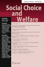
As Fig. 1 illustrates, the family of UC rules is indeed the union of the family of UE rules and EC rules. Note that \(UE^{0}\equiv UC^{0}\equiv U,\), \(EC^{1}\equiv UC^{1}\equiv CD\), whereas \(ES\equiv UE^{1}\equiv EC^{0}\equiv UC^{\frac{n-2}{2\left( n-1\right) }}\) is the unique rule belonging to both families.
Fig. 1
Illustration of the first three families. \(\{UC^{\lambda }\}=\{UE^{\lambda }\}\cup \{EC^{\lambda }\}\)
×
We could generalize the previous families by considering any linear (but not necessarily convex) combination between U and CD, which we shall sometimes refer as generalized compromise rules. Formally,
GUC-family of rules\(\left\{ GUC^{\lambda }\right\} _{\lambda \in {\mathbb {R}}}\): for each \( \lambda \in {\mathbb {R}},\) each \(A\in \mathbf {{\mathcal {P}}}\), and each \(i\in N\) ,
We also consider another category of rules arising from generalizing the equal-split rule to allow for unequal (but fixed) splits of the audience of each game between the two playing teams. Formally,
Split rules\(\left\{ S^{\lambda }\right\} _{\lambda \in \left[ 0,1\right] }\): for each \(\lambda \in \left[ 0,1\right] , \) each \(A \in \mathbf {{\mathcal {P}}}\), and each \(i\in N\),
The equal-split rule corresponds to the case where \(\lambda =0.5.\) The case \(\lambda =0\) corresponds to the rule assigning to each team its home audience and the case \(\lambda =1\) corresponds to the rule assigning to each team its away audience. Thus, we shall refer to each half of the family as home-biased split rules (\(\left\{ S^{\lambda }\right\} _{\lambda \in \left[ 0,\frac{1}{2} \right] }\)) and away-biased split rules (\(\left\{ S^{\lambda }\right\} _{\lambda \in \left[ \frac{1}{2},1\right] }\)), respectively. As before, we could also consider a generalization of the split rules.
Generalized split rules\(\left\{ GS^{\lambda }\right\} _{\lambda \in {\mathbb {R}} }\): for each \(\lambda \in {\mathbb {R}} ,\) each \(A \in \mathbf {{\mathcal {P}}}\), and each \(i\in N,\)
To conclude with this inventory, we consider the most general family of rules encompassing all the rules introduced above. The allocation received by each team i depends on three data: its home audience \(\left( \sum _{j\in N\backslash \left\{ i\right\} }a_{ij}\right) ,\) its away audience \(\left( \sum _{j\in N\backslash \left\{ i\right\} }a_{ji}\right) ,\) and the total audience of the tournament \(\left( \left| \left| A\right| \right| \right) .\) The relative importance of each data is the same for each team. Formally,
General rules \(\left\{ G^{xyz}\right\} _{x+y+nz=1}\). For each trio \(x,y,z\in {\mathbb {R}}\) with \(x+y+nz=1,\) each \( A\in \mathbf {{\mathcal {P}}}\), and each \(i\in N\),
Note that the uniform rule corresponds to the case in which \(x=0,\)\( y=0\) and \(z=\frac{1}{n}.\) The equal-split rule corresponds to the case in which \(x=\frac{1}{2},\)\(y=\frac{1}{2}\) and \(z=0.\)Concede-and-divide corresponds to the case in which \(x=\frac{n-1}{n-2},\)\(y= \frac{n-1}{n-2}\) and \(z=\frac{-1}{n-2}.\) Thus, all GUC rules belong to this family. Besides, generalized split rules also belong to this family (they are obtained when \(x=1-\lambda ,\)\(y=\lambda \) and \(z=0).\)
The family of general rules also contains rules outside the previous families. An interesting example is the following:
which corresponds to \(\left( x,y,z\right) =\left( \frac{-n+1}{2},\frac{-n+1}{ 2},1\right) \). With this rule, the larger the audience of a team, the smaller the revenue it receives. In particular, a team with null audience receives all the revenue.
2.2 Axioms
We now introduce the axioms we consider in this paper.
The first axiom says that if two teams have the same audiences, when facing each of the other teams, then they should receive the same amount.
Equal treatment of equals \(\left( ETE\right) \): For each \(A\in {\mathcal {P}}\), and each pair \(i,j\in N\) such that \(a_{ik}=a_{jk}\), and \( a_{ki}=a_{kj}\), for each \(k\in N{\setminus} \{i,j\}\),
Now, we may want to require something more to consider two teams as truly equals. To wit, the two teams have the same audiences, not only when facing each of the other teams, but also when facing themselves at each stadium. The next axiom only guarantees that they receive the same amount when this extra condition holds.
Weak equal treatment of equals \(\left( WETE\right) \): For each \( A\in {\mathcal {P}}\), and each pair \(i,j\in N\) such that \(a_{ij}=a_{ji},\)\( a_{ik}=a_{jk}\), and \(a_{ki}=a_{kj}\), for each \(k\in N{{\setminus} } \{i,j\}\),
Obviously, this axiom is weaker than the previous one. The following axiom fills the gap. It says that a redistribution between the audiences of the two games involving a pair of teams does not affect the revenues obtained by the teams in the pair.
Pairwise reallocation proofness \(\left( PRP\right) \): For each pair \(A,A^{\prime }\in {\mathcal {P}}\), and each pair \(i_{0},j_{0}\in N\), such that \( a_{ij}=a_{ij}^{\prime }\), for each pair \(\left\{ i,j\right\} \ne \{i_{0},j_{0}\}\), and \(a_{i_{0}j_{0}}+a_{j_{0}i_{0}}=a_{i_{0}j_{0}}^{\prime }+a_{j_{0}i_{0}}^{\prime }\),
$$\begin{aligned} R_{k}(A)=R_{k}(A^{\prime })\text { for each }k=i_{0},j_{0}. \end{aligned}$$
A somewhat related axiom refers to situations where only games played by a pair of teams have a positive audience. It says that the total audience should be allocated to such two teams.
Stand-alone pair \(\left( SAP\right) \): For each \(A\in {\mathcal {P}}\) and each pair \(i,j\in N\) such that \(a_{kl}=0\) for each pair \(\left\{ k,l\right\} \in N\) with \((k,l)\ne (i,j)\) and \((k,l)\ne (j,i)\),
We could instead consider that, for those situations, the remaining teams obtain a homogeneous amount.
Homogeneous effect of stand-alone pair \(\left( HSAP\right) \): For each \(A\in {\mathcal {P}}\) and each pair \(i,j\in N\) such that \(a_{kl}=0\) for each pair \(\left\{ k,l\right\} \in N\), such that \((k,l)\ne (i,j)\) and \( (k,l)\ne (j,i)\),
$$\begin{aligned} R_{k}(A)=R_{l}(A)\text { for each }k,l\in N\backslash \left\{ i,j\right\} . \end{aligned}$$
A strengthening of stand-alone pair says that if a team has null audience, then it gets no revenue. Formally,
Null team \(\left( NT\right) \): For each \(A\in {\mathcal {P}}\), and each \(i\in N\), such that for each \(j\in N\), \(a_{ij}=0=a_{ji}\),
$$\begin{aligned} R_{i}(A)=0. \end{aligned}$$
The following axiom strengthens equal treatment of equals by saying that if the audience of team i is, game by game, not smaller than the audience of team j, then that team i should not receive less than team j.
Order preservation \(\left( OP\right) \): For each \(A\in {\mathcal {P}}\) and each pair \(i,j\in N\), such that, for each \(k\in N\backslash \left\{ i,j\right\} \), \(a_{ik}\ge a_{jk}\) and \(a_{ki}\ge a_{kj}\),
Alternatively, we can consider the natural weaker versions, aligned with weak equal treatment of equals, when also paying attention to the two games involving the pair.
Home order preservation \(\left( HOP\right) \): For each \(A\in {\mathcal {P}}\) and each pair \(i,j\in N\), such that, for each \(k\in N\backslash \left\{ i,j\right\} \), \(a_{ik}\ge a_{jk}\), \(a_{ki}\ge a_{kj}\), and \( a_{ij}\ge a_{ji}\),
Away order preservation \(\left( AOP\right) \): For each \(A\in {\mathcal {P}}\) and each pair \(i,j\in N\), such that, for each \(k\in N\backslash \left\{ i,j\right\} \), \(a_{ik}\ge a_{jk}\), \(a_{ki}\ge a_{kj}\), and \( a_{ji}\ge a_{ij}\),
The next proposition, whose straightforward proof we omit, summarizes the relations between the axioms introduced above.
Proposition 1
The following implications among axioms hold:
1.
Equal treatment of equals implies weak equal treatment of equals.
2.
The combination of weak equal treatment of equals and pairwise reallocation proofness implies equal treatment of equals.
3.
Order preservation implies home order preservation and away order preservation.
4.
The combination of home order preservation (or away order preservation) and pairwise reallocation proofness implies order preservation.
5.
Order preservation implies equal treatment of equals.
6.
Home order preservation (or away order preservation) implies weak equal treatment of equals.
7.
Null team implies stand-alone pair.
8.
Non negativity implies weak upper bound.
9.
Maximum aspirations implies weak upper bound.
3 Characterization results
We consider two subsections. In the first one, we combine weak equal treatment of equals with some other axioms. In the second one, we perform a similar analysis replacing weak equal treatment of equals with weak order preservation.
3.1 With weak equal treatment of equals
Our first result provides several characterizations of the split rules. More precisely, Theorem 1 states that those rules are characterized combining additivity, weak equal treatment of equals and stand-alone pair with one of the three bounds axioms: maximum aspirations, non-negativity or weak upper bound.
Theorem 1
A rule satisfiesadditivity, weak equal treatment of equals, stand-alone pair, and eithermaximum aspirations, non-negativityorweak upper boundif and only if it is a split rule.
As all split rules satisfy null team, and null team implies stand-alone pair (the seventh statement of Proposition 1), we obtain the following corollary from Theorem 1.
Corollary 1
A rule satisfiesadditivity, weak equal treatment of equals, null team, and eithermaximum aspirations, non-negativityorweak upper boundif and only if it is a split rule.
As the next result states, to replace stand-alone pair by pairwise reallocation proofness in Theorem 1 yields a completely different outcome. Instead of split rules, we obtain generalized compromise rules. As a matter of fact, each of the bounds axioms leads to a subfamily of \(GUC^{\lambda }\), arising from considering that \(\lambda \) ranges within a certain interval. More precisely, maximum aspirations leads to the interval \(\left[ \frac{ n-2}{2\left( n-1\right) },1\right] \), non-negativity to the interval \(\left[ \frac{-1}{n-1},\frac{n-2}{ 2\left( n-1\right) }\right] \) and weak upper bound to the interval \( \left[ 1-\frac{n}{2},1\right] \).
Theorem 2
The following statements hold:
1.
A rule satisfiesadditivity, weak equal treatment of equals, pairwise reallocation proofnessandmaximum aspirationsif and only if it belongs to theEC-family of rules.
2.
A rule satisfiesadditivity, weak equal treatment of equals, pairwise reallocation proofnessandnon-negativityif and only if it belongs to theGUC-family of rulesfor\(\lambda \in \left[ \frac{-1}{n-1},\frac{n-2}{2\left( n-1\right) }\right] \).
3.
A rule satisfiesadditivity, weak equal treatment of equals, pairwise reallocation proofnessandweak upper boundif and only if it belongs to theGUC-family of rulesfor\( \lambda \in \left[ 1-\frac{n}{2},1\right] \).
It turns out that dismissing all bounds axioms (maximum aspirations, non-negativity or weak upper bound) in the above results leads to the characterization of the two complete families of generalized (split or compromise) rules.
Theorem 3
The following statements hold:
1.
A rule satisfiesadditivity, weak equal treatment of equalsand eitherstand-alone pair or null teamif and only if it belongs to the family of generalized split rules.
2.
A rule satisfiesadditivity, weak equal treatment of equalsandpairwise reallocation proofnessif and only if it belongs to theGUC-family of rules.
The equal-split rule is the unique rule satisfying additivity, equal treatment of equals and null team (e.g., Bergantiños and Moreno-Ternero 2020a). The first statement of Theorem 3 says that if we replace equal treatment of equals by weak equal treatment of equals in that result we obtain the family of split rules instead of the equal-split rule. It also follows from the second statement of Theorem 3 that the only rule satisfying null team within the GUC-family of rules is precisely the equal-split rule.
The next proposition is obtained by replacing weak equal treatment of equals and pairwise reallocation proofness by equal treatment of equals, in Theorem 2 and the second statement of Theorem 3.
Proposition 2
The following statements hold:
1.
A rule satisfiesadditivity, equal treatment of equalsandmaximum aspirationsif and only if it belongs to theEC-family of rules.
2.
A rule satisfiesadditivity, equal treatment of equalsandnon-negativityif and only if it belongs to theGUC-family of rulesfor\(\lambda \in \left[ \frac{-1}{n-1},\frac{n-2}{ 2\left( n-1\right) }\right] \).
3.
A rule satisfiesadditivity, equal treatment of equalsandweak upper boundif and only if it belongs to theGUC-family of rulesfor\(\lambda \in \left[ 1-\frac{n}{2},1\right] \).
4.
A rule satisfiesadditivityandequal treatment of equalsif and only if it belongs to theGUC-family of rules.
The first statement of Proposition 2 is a refinement of Theorem 1 in Bergantiños and Moreno-Ternero (2021a), obtained by replacing equal treatment of equals with an axiom dubbed symmetry, which says that if two teams have the same audiences they receive the same amounts.
In the next theorem we focus on homogenous effect of stand-alone pair. We replace in the statement of Theorem 1stand-alone pair by this new axiom, and we dismiss the bounds axioms. We obtain a characterization of the general rules.
Theorem 4
A rule satisfiesadditivity, weak equal treatment of equalsandhomogenous effect of stand-alone pairif and only if it is a general rule.
In Theorem 1, we obtain the same family of rules when adding either one of the three bounds axioms. This does not happen in Theorem 4. For instance, the rule corresponding to \(\left( x,y,z\right) =\left( 1,1,\frac{-1 }{n}\right) \) satisfies maximum aspirations (and hence weak upper bound) but violates non-negativity. The rule corresponding to \(\left( x,y,z\right) =\left( \frac{1}{4},\frac{1}{4},\frac{1}{2n}\right) ,\) which is \(\frac{1}{2}U+\frac{1 }{2}ES,\) satisfies non negativity (and hence weak upper bound) but violates maximum aspirations. The rule corresponding to \(\left( \frac{-n+1}{2},\frac{ -n+1}{2},1\right) \) satisfies weak upper bound but violates maximum aspirations and non-negativity.
We conclude providing two tables summarizing the results obtained in this section. First, in Table 1, we summarize the results obtained for generalized split rules. We use capital letters for necessary axioms in the characterizations and small letters for axioms that can be exchanged in the characterization (only one of them is necessary). Second, in Table 2, we summarize the results obtained for generalized compromise rules. When we write \(\left[ a,b\right] \) we refer to the family of rules \(\left\{ GUC^{\lambda }:\lambda \in \left[ a,b\right] \right\} \).
We now explore the implications of strengthening (weak) equal treatment of equals to become (weak) order preservation in the above results. On the one hand, we observe that the three characterizations of the split rules become now characterizations of one half of the family; depending on whether they bias the splitting in favor of the home team or the away team.
Theorem 5
The following statements hold:
1.
A rule satisfiesadditivity, home order preservation, stand-alone pair, and eithermaximum aspirations, non-negativity, orweak upper boundif and only if it is a home-biased split rule.
2.
A rule satisfiesadditivity, away order preservation, stand-alone pair, and eithermaximum aspirations, non-negativity, orweak upper boundif and only if it is an away-biased split rule.
As all split rules satisfy null team, and null team implies stand-alone pair (the seventh statement of Proposition 1), we obtain the following corollary from Theorem 5.
Corollary 2
The following statements hold:
1.
A rule satisfiesadditivity, home order preservation,null team, and eithermaximum aspirations, non-negativityorweak upper boundif and only if it is a home-biased split rule.
2.
A rule satisfiesadditivity, away order preservation,null team, and eithermaximum aspirations, non-negativityorweak upper boundif and only if it is an away-biased split rule.
On the other hand, we obtain characterizations of each of the three families involving convex combinations between the three focal rules; namely, the uniform rule, equal-split rule, and concede-and-divide.
Theorem 6
The following statements hold:
1.
A rule satisfiesadditivity, home order preservationoraway order preservation, pairwise reallocation proofnessandmaximum aspirationsif and only if it belongs to theEC-family of rules.
2.
A rule satisfiesadditivity, home order preservationoraway order preservation, pairwise reallocation proofnessandnon-negativityif and only if it belongs to theUE-family of rules.
3.
A rule satisfiesadditivity, home order preservationoraway order preservation, pairwise reallocation proofnessandweak upper boundif and only if it belongs to theUC-family of rules
As the next result states, dismissing all bounds axioms (maximum aspirations, non-negativity or weak upper bound) in the above results leads to the characterization of half of each of the two complete families of generalized (split or compromise) rules.
Theorem 7
The following statements hold:
1.
A rule satisfiesadditivity, home order preservationand eitherstand-alone pair or null teamif and only if it belongs to theGS-family of rulesfor\(\lambda \le \frac{1}{2}\).
2.
A rule satisfiesadditivity, away order preservationand eitherstand-alone pairornull teamif and only if it belongs to theGS-family of rulesfor\(\lambda \ge \frac{1}{2}\).
3.
A rule satisfiesadditivity, home order preservationoraway order preservationandpairwise reallocation proofnessif and only if it belongs to theGUC-family of rulesfor\(\lambda \ge 0\).
The next proposition is obtained by replacing in Theorem 6, and the last statement of Theorem 7, the combination of home/away order preservation and pairwise reallocation proofness by order preservation.
Proposition 3
The following statements hold:
1.
A rule satisfiesadditivity, order preservationandmaximum aspirationsif and only if it belongs to theEC-family of rules.
2.
A rule satisfiesadditivity, order preservationandnon-negativityif and only if it belongs to theUE-family of rules.
3.
A rule satisfiesadditivity, order preservationandweak upper boundif and only if it belongs to theUC-family of rules.
4.
A rule satisfiesadditivityandorder preservationif and only if it belongs to theGUC-family of rulesfor\(\lambda \ge 0\).
We conclude providing two tables summarizing the results obtained in this section. First, in Table 3, we summarize the results obtained for generalized split rules. When we write \(\left[ a,b\right] \) we refer to the family of rules \(\left\{ GS^{\lambda }:\lambda \in \left[ a,b \right] \right\} \). We use capital letters for necessary axioms in the characterizations and small letters for axioms that can be exchanged in the characterization (only one of them is necessary). Second, in Table 4, we summarize the results obtained for generalized compromise rules. When we write \(\left[ a,b\right] \) we refer to the family of rules \(\left\{ GUC^{\lambda }:\lambda \in \left[ a,b\right] \right\} \).
Table 3
Further characterizations of generalized split rules
We have explored in this paper the axiomatic approach to the problem of sharing the revenues raised from the collective sale of broadcasting rights in sports leagues. We have mostly focussed on two alternative axioms formalizing the notion of impartiality: equal treatment of equals and weak equal treatment of equals. These two axioms, when combined with additivity and some other basic axioms, lead towards two alternative categories of rules. To wit, the former leads to several families of rules compromising between focal existing rules: the uniform rule, the equal-split rule and concede-and-divide. The latter instead leads to a unique family generalizing the equal-split rule to allow for unequal (but fixed) sharing of the audience of each game between the home team and the away team. The choice between equal treatment of equals and weak equal treatment of equals is ultimately a choice between disregarding the effect of \(a_{ij}\ne a_{ji} \) or not and, as such, it is reflected in the characterization results just summarized.
We also characterize a more general family of rules (encompassing all of the above) by combining additivity, weak equal treatment of equals and a third axiom dubbed homogeneous effect of stand-alone pair, which states that in situations where only games played by a pair of teams have a positive audience, the remaining teams obtain a homogeneous amount. In the resulting family, the amount each team receives depends on three numbers: the overall home audience of the team, the overall away audience of the team, and the total audience of the whole tournament. There is a weighted aggregation of these three numbers and the weights are the same for each team.
We have also obtained further characterizations upon strengthening the axioms of equal treatment of equals to become axioms of order preservation in the previous results. In one case, that leads precisely towards convex combinations of the three focal rules. In the other case, to home-biased (or away-biased) split rules, which prioritize home teams (or away teams) in the splitting process within each pair of teams for the games they play.
Common to all of our characterization results is the axiom of additivity. This is an invariance requirement with a long tradition in axiomatic work (e.g., Shapley 1953) but also considered strong under some circumstances. For results without additivity in this model, the reader is referred to Bergantiños and Moreno-Ternero (2020b).
As mentioned above, our analysis is restricted to a fixed-population setting. A generalization to a variable-population setting is left for further research. In such a setting, one would expect that focal axioms such as consistency, or population monotonicity, would play a major role to obtain new characterization results.
To conclude, we mention that one could also be interested into approaching our problems with a (cooperative) game-theoretical approach, a standard approach in many related models of resource allocation (e.g., Littlechild and Owen 1973; van den Nouweland et al. 1996; Ginsburgh and Zang 2003; Bergantiños and Moreno-Ternero 2015). In Bergantiños and Moreno-Ternero (2020a), we associate to our problems a natural optimistic cooperative TU game in which, for each subset of teams, we define its worth as the total audience of the games played by the teams in that subset.8 For such a resulting game, only two-player coalitions have nonzero dividends. Thus, it follows that the Shapley value coincides with the \(\tau \)-value and the nucleolus (e.g., Deng and Papadimitriou 1994; van den Nouweland et al. 1996). All those values yield the same solutions as the equal-split rule for the original problem.9 The egalitarian value (e.g., van den Brink 2007) of that game yields the same solutions as the uniform rule. Casajus and Huettner (2013), van den Brink et al. (2013) and Casajus and Yokote (2019) characterize the family of values arising from the convex combination of the Shapley value and the egalitarian value. In our setting, this would correspond to the family of rules compromising (via convex combinations) between the equal-split rule and the uniform rule. Thus, the second statement of Proposition 3 in our paper could be considered as a parallel result to some of the results in that literature. One could conceivably go beyond convex combinations to consider linear combinations of the Shapley value and the egalitarian value. If so, the resulting generalized egalitarian Shapley values could be associated to our entire family of generalized compromise rules (including concede-and-divide as a member). Finally, the so-called egalitarian nonseparable contribution value (e.g., Driessen and Funaki 1991) of that game yields the same solutions as the dual of the uniform rule, i.e., the rule that imposes to each team a uniform loss (where loss is understood as the difference between claim and obtained amount).10 Thus, the family of values arising from the convex combination of the egalitarian value and the egalitarian nonseparable contribution value (e.g., van den Brink et al. 2016) would correspond in our setting to the family of rules compromising (via convex combinations) between the uniform rule and its dual.
Nevertheless, the game-theoretical approach, although both natural and tractable, is not without loss of generality. For example, one may consider that being a member of a league also involves significant externalities, so that a subgroup of teams may not necessarily achieve the same audiences when part of a smaller league. This, together with the fact that there is not a unique way to associate a TU-game to our problems, leads us to prefer the axiomatic approach to the game-theoretical approach to analyze our problems. That is why we have endorsed the axiomatic approach in this paper.
Acknowledgements
We thank François Maniquet (Managing Editor of this journal), two anonymous referees, and participants at the International Seminar on Social Choice, ICAE Webinars, UPO-ECON Webinars, Korea University Micro Seminar Series, CIO Webinars, University of Arizona FC-Talks (in Memory of Patrick Harless), Riccardo Faini CEIS Webinar, the 2021 SAET Conference and the 2021 International Conference on Social Choice and Voting Theory for helpful comments and suggestions. Financial support from the Spanish Ministry of Economics and Competitiveness, through the research projects ECO2017-82241-R, ECO2017-83069-P, and PID2020-115011GB-I00, Xunta de Galicia through Grant ED431B 2019/34 and Junta de Andalucía through Grant P18-FR-2933 is gratefully acknowledged.
Open AccessThis article is licensed under a Creative Commons Attribution 4.0 International License, which permits use, sharing, adaptation, distribution and reproduction in any medium or format, as long as you give appropriate credit to the original author(s) and the source, provide a link to the Creative Commons licence, and indicate if changes were made. The images or other third party material in this article are included in the article's Creative Commons licence, unless indicated otherwise in a credit line to the material. If material is not included in the article's Creative Commons licence and your intended use is not permitted by statutory regulation or exceeds the permitted use, you will need to obtain permission directly from the copyright holder. To view a copy of this licence, visit http://creativecommons.org/licenses/by/4.0/.
Publisher's Note
Springer Nature remains neutral with regard to jurisdictional claims in published maps and institutional affiliations.
For ease of exposition, we present the proofs of the results in a different order. In most of the proofs, we shall make use of the following notation. For each pair \(i,j\in N\), with \(i\ne j\), let \({\varvec{1}}^{ij}\) denote the matrix with the following entries:
It is straightforward to show that each generalized split rule satisfies additivity, weak equal treatment of equals, stand-alone pair and null team. Conversely, let R be a rule satisfying additivity, weak equal treatment of equals and either stand-alone pair or null team. Let \(i,j\in N\) with \(i\ne j\). By weak equal treatment of equals, there exists \(z^{ij}\in {\mathbb {R}}\) such that \(R_{k}\left( {\varvec{1}} ^{ij}\right) =z^{ij}\) for all \(k\in N\backslash \left\{ i,j\right\} .\) Let \( R_{i}\left( {\varvec{1}}^{ij}\right) =x^{ij}\) and \(R_{j}\left( \varvec{ 1}^{ij}\right) =y^{ij}\). Then, \(x^{ij}+y^{ij}+(n-2)z^{ij}=||{\varvec{1}} ^{ij}||=1\).
By stand-alone pair or null team, \(z^{ij}=0\) and \(y^{ij}=1-x^{ij}\).
By weak equal treatment of equals, \(1-x^{ij}=1-x^{ik}\). Hence, \( x^{ij}=x^{ik}\).
Therefore, for each \(i\in N\) there exists \(x_{i}\in {\mathbb {R}}\) such that \( R_{i}\left( {\varvec{1}}^{ij}\right) =x_{i}\), for each \(j\in N\). Thus,
By weak equal treatment of equals, \(x_{i}+1-x_{j}=1-x_{i}+x_{j}\). Hence, \(x_{i}=x_{j}\). Thus, \(R_{i}\left( {\varvec{1}}^{ij}\right) =x\), for each pair \(i,j\in N\).
Finally, let \(A\in {\mathcal {P}}\) and \(i\in N.\) By additivity,
It is straightforward to show that each split rule satisfies all the axioms in the statement. Conversely, let R be a rule that satisfies additivity, weak equal treatment of equals, stand-alone pair, and either maximum aspirations, non-negativity or weak upper bound. By the first statement of Theorem 3, there exists \(\lambda \in {\mathbb {R}}\) such that \(R(A)=GS^{\lambda }\left( A\right) .\)
Let \(i,j\in N\) with \(i\ne j.\)
By maximum aspirations, \(1-\lambda =R_{i}\left( {\varvec{1}} ^{ij}\right) \le \alpha _{i}\left( {\varvec{1}}^{ij}\right) =1,\) and \( \lambda =R_{j}\left( {\varvec{1}}^{ij}\right) \le \alpha _{j}\left( {\varvec{1}}^{ij}\right) =1.\)
By non-negativity, \(1-\lambda =R_{i}\left( {\varvec{1}} ^{ij}\right) \ge 0,\) and \(\lambda =R_{j}\left( {\varvec{1}}^{ij}\right) \ge 0.\)
It is obvious that U and CD satisfy additivity and equal treatment of equals. Then, each rule within the GUC-family also satisfies the two axioms. Conversely, let R be a rule satisfying additivity and equal treatment of equals. Let \(i,j\in N\) with \(i\ne j.\) By equal treatment of equals, there exist \(x^{ij},z^{ij}\in {\mathbb {R}}\) such that \(R_{i}\left( \varvec{ 1}^{ij}\right) =R_{j}\left( {\varvec{1}}^{ij}\right) =x^{ij}\) and \( R_{k}\left( {\varvec{1}}^{ij}\right) =z^{ij}=\frac{1-2x^{ij}}{n-2}\) for all \(k\in N\backslash \left\{ i,j\right\} \).
By equal treatment of equals, \(R_{j}\left( {\varvec{1}}^{ij}+ {\varvec{1}}^{ik}\right) =R_{k}\left( {\varvec{1}}^{ij}+{\varvec{1}} ^{ik}\right) \). Thus, \(x^{ij}+\frac{1-2x^{ik}}{n-2}=x^{ik}+\frac{1-2x^{ij}}{ n-2}\), which implies that \(x^{ij}=x^{ik}\). Therefore, there exists \(x\in {\mathbb {R}}\) such that for each \(\left\{ i,j\right\} \subset N,\)
Thus, \(R\left( {\varvec{1}}^{ij}\right) =GUC^{\lambda }\left( \varvec{1 }^{ij}\right) \). As both rules satisfy additivity, we deduce from here that \(R\left( A\right) =GUC^{\lambda }(A)\), for each \(A\in {\mathcal {P}}\) , as desired.
By the fourth statement of Proposition 2, each rule within the EC-family satisfies additivity and equal treatment of equals. It is straightforward to show that they also satisfy maximum aspirations. Conversely, let R be a rule satisfying those three axioms. By the fourth statement of Proposition 2, there exists \(\lambda \in {\mathbb {R}}\) such that \(R=GUC^{\lambda }\).
Let \(i,j\in N\) with \(i\ne j.\) By maximum aspirations,
It then follows that \(\lambda \) ranges from \(\frac{n-2}{2(n-1)}\) to 1. As \( UC^{\lambda }\equiv ES\), when \(\lambda =\frac{n-2}{2\left( n-1\right) }\), this concludes the proof of this statement.
By the fourth statement of Proposition 2, each rule from the statement satisfies additivity and equal treatment of equals. As for non-negativity, one can also show (after some algebraic computations) that, for each \(\lambda \in \left[ \frac{-1}{n-1},\frac{n-2}{ 2\left( n-1\right) }\right] \), \(GUC^{\lambda }\) satisfies it too. Conversely, let R be a rule satisfying those three axioms. By the fourth statement of Proposition 2, there exists \(\lambda \in {\mathbb {R}} \) such that \(R=GUC^{\lambda }\).
Let \(i,j\in N\) with \(i\ne j.\) By non-negativity,
It then follows that \(\lambda \) ranges from \(\frac{-1}{n-1}\) to \(\frac{n-2}{ 2\left( n-1\right) }\) to 1, which concludes the proof of this statement.
By the fourth statement of Proposition 2, each rule from the statement satisfies additivity and equal treatment of equals. As for weak upper bound, one can also show (after some algebraic computations) that, for each \(\lambda \in \left[ 1-\frac{n}{2},1\right] \), \( GUC^{\lambda }\) satisfies it too. Conversely, let R be a rule satisfying those three axioms. By the fourth statement of Proposition 2, there exists \(\lambda \in {\mathbb {R}} \) such that \(R=GUC^{\lambda }\).
Let \(i,j\in N\) with \(i\ne j.\) By weak upper bound,
It is straightforward to show that each rule within the GUC-family satisfies pairwise reallocation proofness. Then, each statement of Theorem 2 follows from the corresponding statement at Proposition 2, together with the first two statements of Proposition 1.
It is straightforward to show that each general rule satisfies the three axioms in the statement. Conversely, let R be a rule satisfying the three axioms. Let \(i,j\in N\) with \(i\ne j\). By weak equal treatment of equals, there exists \(z^{ij}\in {\mathbb {R}}\) such that \(R_{k}\left( {\varvec{1}}^{ij}\right) =z^{ij}\) for all \(k\in N\backslash \left\{ i,j\right\} .\) Let \(R_{i}\left( {\varvec{1}}^{ij}\right) =x^{ij}\) and \( R_{j}\left( {\varvec{1}}^{ij}\right) =y^{ij}\). Then, \( x^{ij}+y^{ij}+(n-2)z^{ij}=||{\varvec{1}}^{ij}||=1\).
By weak equal treatment of equals, \(y^{ij}+z^{ik}=z^{ij}+y^{ik}\). Hence, \(y^{ij}-z^{ij}=y^{ik}-z^{ik}.\) Thus, \(y^{i}=y^{ij}-z^{ij}\) is well defined (does not depend on j). Now, for each \(i,j\in N,\)\( y^{ij}=z^{ij}+y^{i}.\)
By weak equal treatment of equals, \(x^{ji}+z^{ki}=z^{ji}+x^{ki}\). Hence, \(x^{ji}-z^{ji}=x^{ki}-z^{ki}.\) Thus, \(x^{i}=x^{ij}-z^{ij}\) is well defined (does not depend on j). Now, for each \(i,j\in N,\)\( x^{ij}=z^{ij}+x^{i}.\)
Let \(i,j,k\in N\) with \(i\ne j\) and \(i\ne k.\) Then,
Thus, there exists z such that \(z^{ij}=z\) for all \(i,j\in N.\)
By weak equal treatment of equals, \(R_{i}\left( {\varvec{1}}^{ij}+ {\varvec{1}}^{ji}\right) =R_{j}\left( {\varvec{1}}^{ij}+{\varvec{1}} ^{ji}\right) .\) As
By the first statement of Theorem 3, each generalized split rule satisfies additivity, stand-alone pair and null team. As for home order preservation, let \( A\in {\mathcal {P}}\), and \(i,j\in N\) as in the definition of the axiom. Note that
Now, for each \(k\in N\backslash \left\{ i,j\right\} \), \(GS_{i}^{\lambda }\left( {\varvec{1}}^{ik}\right) =GS_{j}^{\lambda }\left( {\varvec{1}} ^{jk}\right) =1-\lambda \) and \(GS_{i}^{\lambda }\left( {\varvec{1}} ^{ki}\right) =GS_{j}^{\lambda }\left( {\varvec{1}}^{kj}\right) =\lambda \). Similarly, \(GS_{i}^{\lambda }\left( {\varvec{1}}^{kl}\right) =GS_{j}^{\lambda }\left( {\varvec{1}}^{kl}\right) =0\), for each pair \( k,l\in N\backslash \left\{ i,j\right\} \). Finally, \(a_{ij}GS_{i}^{\lambda }\left( {\varvec{1}}^{ij}\right) +a_{ji}GS_{i}^{\lambda }\left( {\varvec{1}}^{ji}\right) \ge a_{ij}GS_{j}^{\lambda }\left( {\varvec{1}} ^{ij}\right) +a_{ji}GS_{j}^{\lambda }\left( {\varvec{1}}^{ji}\right) \) if and only if \(\left( a_{ij}-a_{ji}\right) \left( 1-2\lambda \right) \ge 0\). As \(\lambda \le \)\(\frac{1}{2}\), \(GS_{i}^{\lambda }\left( A\right) \ge GS_{j}^{\lambda }\left( A\right) \), as desired. Likewise, for each \(\lambda \ge \)\(\frac{1}{2}\), \(GS^{\lambda }\) satisfies away order preservation.
Conversely, let R be a rule satisfying additivity, either home order preservation or away order preservation, and either stand-alone pair or null team. By the sixth statement of Proposition 1, R also satisfies weak equal treatment of equals. Thus, by the first statement of Theorem 3, there exists \(\lambda \in {\mathbb {R}}\) such that \( R=GS^{\lambda }.\) Then, for each pair \(i,j\in N\) such that \(i\ne j\), \( R_{i}\left( {\varvec{1}}^{ij}\right) =1-\lambda \) and \(R_{j}\left( {\varvec{1}}^{ij}\right) =\lambda \). Now, if R satisfies home order preservation, \(1-\lambda =R_{i}\left( {\varvec{1}}^{ij}\right) \ge R_{j}\left( {\varvec{1}}^{ij}\right) =\lambda \). Thus, \(\lambda \in \left( -\infty ,\frac{1}{2}\right] \), which concludes the proof of the first statement. Likewise, if R satisfies away order preservation, \( 1-\lambda =R_{i}\left( {\varvec{1}}^{ij}\right) \le R_{j}\left( {\varvec{1}}^{ij}\right) =\lambda \). Thus, \(\lambda \in \left[ \frac{1}{2}, +\infty \right) \), which concludes the proof of the second statement.
Except for the weak order preservation axioms, we already know from Theorem 1 that each split rule satisfies all the axioms in the statement. By the first two statements of Theorem 7, each home-biased split rule satisfies home order preservation and each away-biased split rule satisfies away order preservation. Conversely, let R be a rule satisfying additivity, either home order preservation or away order preservation, stand-alone pair, and either maximum aspirations, non-negativity, or weak upper bound. By the sixth statement of Proposition 1, R also satisfies weak equal treatment of equals. Thus, by Theorem 1, there exists \(\lambda \in [0,1]\) such that \( R=S^{\lambda }.\) In particular, for each pair \(i,j\in N\) such that \(i\ne j\) , \(R_{i}\left( {\varvec{1}}^{ij}\right) =1-\lambda \) and \(R_{j}\left( {\varvec{1}}^{ij}\right) =\lambda \). Now, if R satisfies home order preservation, \(1-\lambda =R_{i}\left( {\varvec{1}}^{ij}\right) \ge R_{j}\left( {\varvec{1}}^{ij}\right) =\lambda \). Thus, \(\lambda \in \left[ 0,\frac{1}{2}\right] \), which concludes the proof of the first statement. Likewise, if R satisfies away order preservation, \(1-\lambda =R_{i}\left( {\varvec{1}}^{ij}\right) \le R_{j}\left( {\varvec{1}} ^{ij}\right) =\lambda \). Thus, \(\lambda \in \left[ \frac{1}{2},1\right] \), which concludes the proof of the second statement.
We know each rule within the GUC-family satisfies additivity. As concede-and-divide satisfies order preservation, and the uniform rule assigns the same amount to all teams, it follows that \((1-\lambda )U+\lambda CD\) also satisfies order preservation for each \(\lambda \in \left[ 0,\infty \right) \). Conversely, let R be a rule satisfying additivity and order preservation. By the fifth statement of Proposition 1, R also satisfies equal treatment of equals. Thus, by the fourth statement of Proposition 2, there exists \(\lambda \in {\mathbb {R}}\) such that \( R=GUC^{\lambda }.\) Besides, given \(i,j\in N\) with \(i\ne j,\)
$$\begin{aligned} R_{k}\left( {\varvec{1}}^{ij}\right) =\left\{ \begin{array}{cc} x &{}\quad \hbox { if }k=i,j \\ \frac{1-2x}{n-2} &{}\quad \hbox { otherwise.} \end{array} \right. \end{aligned}$$
By order preservation, \(x\ge \frac{1-2x}{n-2}\) which implies that \( x\ge \frac{1}{n}\). As \(\lambda =\frac{nx-1}{n-1}\), it follows that \(\lambda \in \left[ 0,+\infty \right) .\)
As mentioned above, each rule within the EC-family satisfies additivity and maximum aspirations. It is obvious that ES and CD satisfy order preservation. Then, each rule within the EC-family satisfies order preservation. Conversely, let R be a rule satisfying those three axioms. By the fourth statement of Proposition 3, there exists \(\lambda \in \left[ 0,+\infty \right) \) such that \( R=GUC^{\lambda }\). By maximum aspirations, similarly to the proof of the first statement of Proposition 2, we can conclude that \( \lambda \)\(\in \left[ \frac{n-2}{2(n-1)},1\right] .\) Namely, R belongs to the EC-family, as desired.
As mentioned above, each rule within the UE-family satisfies additivity and non-negativity. As U and ES satisfy order preservation, each rule within the UE-family satisfies it too. Conversely, let R be a rule satisfying those three axioms. By the fourth statement of Proposition 3, there exists \( \lambda \in \left[ 0,+\infty \right) \) such that \(R=GUC^{\lambda }\). By non negativity, similarly to the proof of the second statement of Proposition 2, we can conclude that \(\lambda\,\in \left[ 0, \frac{n-2}{2(n-1)}\right].\) Namely, R belongs to the UE-family, as desired.
As mentioned above, each rule within the UC-family satisfies additivity and weak upper bound. It is obvious that U and CD satisfy order preservation. Then, each rule within the UC-family satisfies order preservation. Conversely, let R be a rule satisfying those three axioms. By the fourth statement of Proposition 3, there exists \(\lambda \in \left[ 0,+\infty \right) \) such that \(R=GUC^{\lambda }\). By weak upper bound, similarly to the proof of the third statement of Proposition 2, we can conclude that \( \lambda \in \left[ 0,1\right] \). Namely, R belongs to the UC-family, as desired.
This result is almost equivalent to the characterization in Bergantiños and Moreno-Ternero (2021a). Therein, we use a stronger notion than equal treatment of equals indicating that two teams with the same claims receive the same awards.
We are therefore assuming a round-robin tournament in which each team plays in turn against each other team twice: once home, another away. This is the usual format of the main European football leagues. Our model could also be extended to leagues in which some teams play other teams a different number of times and play-offs at the end of the regular season, which is the usual format of North American professional sports. In such a case, \(a_{ij}\) is the broadcasting audience in all games played by i and j at i’s stadium.
This interesting principle of comparing individual performance with average performance is often used in other contexts (e.g., Arrfelt et al. 2013; Allen et al. 2017; Ju et al. 2021).
Alternative natural options could also be considered in order to construct a characteristic function leading to a TU-game associated to our problems. To do so, one has to take a stance on what revenue a coalition can generate on its own. It is not obvious that any coalition of teams can generate the broadcasting revenues its members generated while being members of the league (the grand coalition). The above is an “optimistic” option assuming that each coalition of teams can generate the broadcasting revenues its members generated while being members of the league.
The property that only two-player coalitions have nonzero dividends is used by Maniquet (2003), who shows that the so-called minimal transfer rule for queueing problems coincides with the Shapley value of the associated TU-game. As mentioned above, it follows from the property that coincidence with the nucleolus of such a game also holds, which is shown directly by Chun and Hokari (2007).
This is actually a specific convex combination between the equal-split rule and concede-and-divide, thus satisfying additivity, equal treatment of equals (as a matter of fact, order preservation) and maximum aspirations. As the number of teams becomes large, the convex combination approaches concede-and-divide.