We consider an odd-sized “jury”, which votes sequentially between two equiprobable states of Nature (say A and B, or Innocent and Guilty), with the majority opinion determining the verdict. Jurors have private information in the form of a signal in \([-1,+1]\), with higher signals indicating A more likely. Each juror has an ability in [0, 1], which is proportional to the probability of A given a positive signal, an analog of Condorcet’s p for binary signals. We assume that jurors vote honestly for the alternative they view more likely, given their signal and prior voting, because they are experts who want to enhance their reputation (after their vote and actual state of Nature is revealed). For a fixed set of jury abilities, the reliability of the verdict depends on the voting order. For a jury of size three, the optimal ordering is always as follows: middle ability first, then highest ability, then lowest. For sufficiently heterogeneous juries, sequential voting is more reliable than simultaneous voting and is in fact optimal (allowing for non-honest voting). When average ability is fixed, verdict reliability is increasing in heterogeneity. For medium-sized juries, we find through simulation that the median ability juror should still vote first and the remaining ones should have increasing and then decreasing abilities.
Hinweise
Publisher's Note
Springer Nature remains neutral with regard to jurisdictional claims in published maps and institutional affiliations.
1 Introduction
This paper extends the Condorcet jury theory to juries that vote sequentially (knowing earlier votes) rather than simultaneously. Since we consider jurors who are heterogenous with respect to their ability to determine the true state of Nature (equiprobably A or B, Innocent or Guilty), it turns out that the order in which they vote affects the reliability of the majority verdict. By reliability we simply mean the probability that the majority verdict agrees with the actual state of Nature. We prove that for a jury of size three with any fixed abilities, the voting order with greatest reliability is median ability first, then highest ability, then lowest. Using simulation, we suggest that, for medium-sized juries, the median ability juror should still vote first. Then the abilities should increase, and after the highest ability juror votes, the rest should vote in decreasing order. An intuition for this is that if the highest-ability juror votes first, then herding may reduce the contribution of the others; if he votes last, then the majority verdict may be decided before he even gets to vote.
In a model where jurors have private information in the form of a binary signal (A or B), Condorcet showed that for jurors of common ability \(p>1/2\) (probability of a correct signal), or of varying abilities all at least p, the reliability approaches 1 as the jury size increases.
Anzeige
Our model is a little more sophisticated than that of Condorcet in two ways: signals and abilities. Condorcet’s voters get a binary signal, for A or for B. Our jurors get a signal s in the interval \([-1,+1]\), with higher signals giving a higher probability of A. The signal \(s=0\) is neutral and useless, as A and B remain equally likely after such a signal. In analogy with Condorcet’s probability p (that the binary signal is correct) our jurors have an ability in the interval [0, 1], which is proportional to the probability of A given a positive signal s, \(0<s\le 1\). An ability of 0 makes that probability 1/2, the same as the a priori probability and hence useless (no ability at all). Jurors of higher ability have, in general, more useful private information. When a juror of given ability comes to vote, he will vote for the alternative, A or B, that he views as more likely, given prior voting and his private signal s. This type of voting, called honest voting, models the jurors as experts who have known abilities by reputation. They wish to vote for the alternative that turns out to be true, assuming Nature is eventually revealed. This would be true if they are making short term predictions (say weather or the economy). This type of voting by experts was introduced by Ottaviani and Sørensen (2001), although they do not employ a majority verdict, which we will discuss in detail in the next section. Overall, the model of signals and abilities used here is the same linear signal model introduced in Alpern and Chen (2017b) in a simpler voting model and is similar in spirit to the discrete signal and ability model of Alpern and Chen (2017a), which is unique in some sense (Alpern et al. 2021). The way in which a juror’s signal and ability affect his judgement of the probability of A is described fully in Sect. 4.
Given the above model, we are able to address four questions about the comparative reliability of different voting schemes or voting orders. The main question addressed in this article is the optimal voting order for jurors of different abilities. Putting higher ability jurors first is more likely to have them vote before a majority verdict is established, but also may create negative herding effects. We also consider when sequential honest voting, where jurors can take into account previous voting, is better or worse than simultaneous voting (or secret ballot)as in the Condorcet model. We also answer the question of whether, for fixed average ability, a more heterogeneous or homogeneous jury has higher reliability when voting in the optimal sequential order. Finally, we ask when sequential honest voting is optimal in that it maximizes the reliability of the verdict. If not, the jurors might be incentivized to jointly modify their voting thresholds to produce a better verdict, which could mean possibly voting for the alternative that a juror views as less likely. This might be accomplished by giving all jurors a reward later, if majority verdict turns out to be correct, or perhaps by giving them stock in the company making the decision. Since we are dealing with majority verdicts and, for a single member jury, all the above distinctions are meaningless, we consider a jury of three experts, where we find sharp answers to all of our above questions.
We note that while electorates in preference voting are typically large, juries in information voting are typically small, and often of size three, such as refereeing team in tennis or boxing, appellate levels in legal decisions, doctors giving second or third opinions on the necessity of an operation. For juries of size three we are able to answer all of our above questions regarding comparative reliability.
This paper is organized as follows. After a literature review in the next section, we present in Sect. 3 some simple results and intuitions under some simplified settings, before formally introducing our model in Sects. 4 and 5. We present our main results in Sects. 6–9, which are summarized as follows:
1.
Optimal order of last two jurors (Theorem 1) For any odd-sized jury, reliability is maximized when the last two jurors vote in decreasing order of ability.
2.
Optimal voting order (Theorem 2) For juries of distinct abilities, the unique voting order that maximizes the reliability of the verdict for honest sequential voting is given as follows: the median ability expert should vote first, then the expert of highest ability, and finally the expert of least ability. [This order was suggested by numerical work in Alpern and Chen (2017a).] This is our main result and by far the hardest to prove. See also the introduction of the more general Ascending–Descending Order (ADO) ordering in Sect. 10: The median ability juror votes first, then the voting is in increasing order up to the highest ability. After the highest votes, the remaining jurors vote in decreasing order of ability.
3.
Monotonicity of reliability in ability (Theorem 3) Abler juries give more reliable verdicts.
4.
Seniority vs. anti-seniority voting orders (Theorem 4) The seniority voting order (decreasing order of ability) has a strictly higher reliability of the verdict than the anti-seniority order (increasing order of ability), unless all jurors have the same ability.
5.
Sequential vs. simultaneous voting (Theorem 5) When the abilities of the jurors are sufficiently homogeneous, simultaneous voting has higher reliability than sequential voting. But when the abilities are sufficiently heterogeneous, honest sequential voting (in the optimal order) has higher reliability. (We provide suitable indices of homogeneity and heterogeneity.)
6.
Effect of diversity on reliability (Theorem 6) For a jury of fixed average ability, reliability is an increasing function of the heterogeneity index.
7.
When is honest sequential voting strategic, that is, (perfectly) optimal? (Theorem 7) When the abilities of the jurors are sufficiently heterogeneous, honest sequential voting in the optimal order is strategic in that it maximizes reliability with respect to any (not just honest) strategy thresholds.
8.
While sequentially voting, if each juror also reveals his signal, what is the optimal order? (Theorem 8) The optimal order of sequential deliberation is the seniority order.
Note that the proofs of all the aforementioned eight theorems are completely independent except that Theorem 2 is based on Theorem 1. The order in which these later results are presented could have been different. In Sect. 10, we consider majority voting of medium-sized juries and propose an analog of the optimal rank ordering of abilities for three-member juries. We complete our paper by making some concluding remarks in Sect. 11.
Anzeige
To see how these results aid an organization that has to make a binary decision, consider that the organization has hired three experts of distinct abilities and wishes to determine the optimal voting mechanism. First, suppose it has no additional funds to incentivize strategic voting, so voting is honest. If the abilities of the fixed set of experts are sufficiently homogeneous, it should keep the voting silent (or simultaneous) by not allowing later voters to know the results of earlier voting (Theorem 5). (This is done for preference voting in US elections, but for different reasons.) If the ability set is sufficiently heterogeneous, then later voters should be told the outcome of earlier votes (Theorem 5) and they should vote in the order given by Theorem 2. We note that other variations are possible, for example, later voters could be told the votes of only some of the earlier voters. If the jury is not fixed, then Theorem 6 suggests that, assuming the cost of an expert juror is increasing in ability, heterogeneous juries might be preferable. Finally, we consider whether it might be advantageous to pay a bonus to each expert for a correct jury (majority) decision, assuming the correctness of the verdict becomes common knowledge in the near future, as with weather predictions. In general, this will be a cost-benefit problem, but Theorem 7 shows that such payments are wasteful if the ability set is sufficiently heterogeneous.
For larger juries of odd size \(n=2m+1\), we propose the Ascending–Descending Order (ADO), where the most able \(m+1\) jurors vote first in increasing ability order and then the least able m jurors vote in descending ability order. We already know from Theorem 2 that ADO is optimal for \(n=3\). Using simulation techniques, we establish that the ADO is an excellent heuristic (and possibly optimal) for \(n=5\) and \(n=7\).
To conclude the section, we remark that our problem can be viewed as a simple optimization problem faced by a decision maker, who has an unordered set of people to form a jury to help him make a binary decision. He wants to arrange their voting order so as to make the majority decision of the jury as reliable as possible. On the other hand, we can also view our problem more game theoretically as a Stackelberg game or principal agent problem. First, we are given an unordered set of jurors. The Principal, who moves first, selects an order in which they must vote. He wins the game (payoff 1; otherwise payoff 0) if the majority verdict is the true state of Nature. Then the jurors vote openly in the order selected by the Principal. In this sub-game, a juror wins (payoff 1; otherwise payoff 0) if his vote is the same as the true state of Nature. That is, the Principal cares only about the correctness of the verdict, while the jurors care only about the correctness of their own votes. In the sub-game, honest voting is exactly the unique Nash equilibrium. In fact, no juror can improve his expected payoff (probability he votes correctly) by changing from honesty, if the prior voters stick to honest voting. Thus it is stronger than the usual definition of Nash equilibrium.
2 Literature
The celebrated Condorcet jury theorem (Condorcet 1785) is concerned with a model with an odd number n of jurors who receive independent binary signals for one of two states of Nature. Each juror receives the correct signal with the same probability p. Condorcet’s Jury theorem (CJT) states that if each juror votes his signal, the probability that the majority vote is correct goes to 1 as n approaches to infinity if \(p>1/2\). There is a large body of literature on extensions and discussions of this result. In this paper we are interested in extensions to sequential voting of heterogeneous ability jurors, where the jurors vote in order, with knowledge of all previous votes. In particularly we are interested in work related to voting order.
In Ottaviani and Sørensen (2001) jurors have heterogeneous abilities (as in this paper), who care only about being right (they are “experts”, with reputations to uphold), rather than about obtaining a correct verdict. We call them honest voters. The main difference between our model and theirs is that our model stays within the Condorcet jury context, where the verdict is simply the majority vote, while their model has a “decision maker” who determines the group decision after all votes have been cast. They talk about the problem of groupthink, herding and conformism, and the last is also discussed in terms of committee decisions regarding the “secretary problem” in Alpern and Baston (2016).
Dekel and Piccione (2000) mainly consider the equilibria of simultaneous versus sequential voting, but they do make an important comment on voting order of heterogeneous jurors” in their Conclusions (p. 48):
“...if voters are endowed ex ante with differential information (some voters can be better informed than others), knowing which voters voted in favor and which against can affect the choice of a later voter. It can be shown that, in a common-value and two signal environment (as in Sec. IIIC above), if the player’s signals are completely ordered (in the sense of Blackwell), then it is optimal to have the better informed vote earlier. This provides an interesting contrast to the findings of Ottaviani and Sørensen (2001). They obtain the opposite optimal order in an environment in which information providers care not about the outcome but about appearing to be well informed. It is not difficult, however, to construct examples in which having the best-informed voter vote first is not optimal. Hence it seems unlikely that general insights into this question can be obtained.”
The point of this paper is that we are indeed able to obtain general insights into this question.
Ali et al. (2008) discuss the optimal voting order of experts and cite examples in which courts of judges follow either anti-seniority (increasing order of ability, in our terminology) or seniority (decreasing order) orders, respectively, in the ancient Sanhedrin court and in the contemporary American Supreme Court. Voting order in selection committees is analyzed in Alpern, Gal and Solan (2010), but there voting is by veto.
A sequential voting model, with discrete but non binary signals, was introduced by Alpern and Chen (2017a). Ability levels were also discrete, so propositions about which ability orderings are best could be obtained by exhaustive search among the finite number of possibilities. Most of that paper is about strategic voting where voters wish to obtain the correct majority verdict, even if this means voting for an alternative which a juror believes to be less likely. For the question of the optimal ability ordering of three jurors with abilities \(a<b<c\), that paper shows by exhaustive search that b, a, c and b, c, a are the optimal orderings (the order of the last two voters in strategic voting does not matter). For honest voting, it is shown for the finite number of cases considered, that the ordering b, c, a is optimal. This is the observation that led us to attempt the general algebraic proof, where a, b and c are real numbers, that is given here. The first algebraic proof of this kind was obtained recently by Alpern and Chen (2017b) for a simpler voting model, where first two jurors vote simultaneously and then the remaining (third) juror casts the deciding vote if there is a tie. This is a much simpler model algebraically as there are only two voting thresholds to consider (for the casting voter), depending on whether the the more able juror voted A or B. Alpern and Chen (2017a) also consider larger juries, up to size 13. It uses simulation to compare randomly generated juries, which vote honestly in increasing, decreasing or random ability order. For all these sizes, decreasing order has higher reliability than random, and random has higher reliability than increasing order.
For a simpler voting model described above with n-1 jurors voting simultaneously, followed by a tie breaking vote (if necessary) of the remaining voter, Alpern and Chen (2017b) showed that for \(n=3\) the voter of median ability should have the casting vote, with honest voting.
A related literature compares the efficacy of sequential versus simultaneous voting. A potential problem with the former is the possibility of herding and information cascades, especially when more able voters are at the beginning of the sequence. Here, voters ignore their own private information to vote instead based on a consensus achieved by earlier voters. On the other hand, with sequential voting each juror has more information to go on. Bikhchandani, Hirshleifer and Welch (1992) explore the probability of informational cascades and also the probability that they converge on an incorrect outcome. They explain many recognized phenomena based on this convergence. In this respect, Ottaviani and Sorensen find that “increasing the quality of some experts on the committee can exacerbate herd behavior and hence decrease the amount of information collected by the decision maker”. A more recent approach to this problem, by computer scientists exploring sequential voting in the context of what are known as social recommendation systems (such as Amazon product valuations, written with knowledge of previous customer’s evaluations) is given by Celis, Krafft and Kobe (2016). They analyze student-reported learning and find that “sequential voting systems can surface better content than systems that elicit independent votes”. A related paper, which deals with sequential evaluations, is Besbes and Scarsini (2018) and considers the possibility of only revealing the mean of prior evaluations. This brings the suggestion of varying our model so that jurors know the prior unascribed vote (such as three votes for A and one for B) without revealing how each prior juror individually voted. This model will be for our future work.
Condorcet theory has also been applied to particular problems: statistical estimation in Pivato (2013), forecasting US election results in Murr (2015) and for project evaluation in Koh (2008). The last of these considers both heterogeneous jurors and voting order.
3 Simple results on sequential juries
As a warm-up, this section serves the purpose of giving some simple results and intuitions for optimally reliable voting orders on heterogeneous sequential juries, without resort to the full continuous signal model mentioned above and defined precisely later in Eq. (3) of Sect. 4. We first consider Condorcet jurors, who are defined as receiving binary signals (for the two possible states of Nature A or B) and then we consider what we call sophisticated jurors, who receive real number signals in the interval \([-1, +1]\).
3.1 Condorcet jurors
We begin with a simple model with three jurors, who we call jurors \(J_1\), \(J_2\) and \(J_3\) in terms of voting order and get correct binary signals \(s\in \{A, B\}\) with probabilities \(p_1\), \(p_2\) and \(p_3\), respectively. We also write \(\{ p_1,p_2, p_3\} =\{p,q,r\}\) where \(p\le q\le r\), and also call the jurors P, Q and R in terms of ability. So if the juror of highest ability votes first, then we have \(J_1\) = R. We similarly label the signals received by the jurors as \(\{s_{1},s_{2},s_{3}\}\) or \(\{s_{p},s_{q},s_{r}\}\). For example, signal \(s_{1}\) is correct with probability \(p_1\). Given the three signals \(\{s_{p},s_{q},s_{r}\}\), it is easy to calculate the most likely state of Nature, which we call the Full Information Solution (FIS). (For a jury of more general jurors than Condorcet, the FIS is expressed in (21).) Clearly, such a state is either \(s_{r}\) (dictator verdict) or \(s_{p}=s_{q} \ne s_r\) (majority verdict). If \(s_{r}=A\) and \(s_{p}=s_{q}=B\), the posterior probability of A is given by
$$\begin{aligned} r \ge {\bar{p}}\equiv \frac{pq}{1-p-q+2pq}. \end{aligned}$$
Proposition 1
The FIS can be obtained from honest sequential majority voting for all ability triples if and only if the highest ability juror votes second.
Proof
If the highest ability juror R votes first (R = \(J_1\)), then \(J_2\) and then \(J_3\) will copy his vote in a cascade. This will fail to choose the FIS if \(r<{\bar{p}}\) and \(J_2\) and \(J_3\) both have the opposite signal to R, since in this case the FIS is \(s_{2}=s_{3}\), while the verdict is \(s_{1}\). If R votes last (R = \(J_3\)) and \(r>{\bar{p}}\), then R’s signal \(s_{r}\) is the FIS. However, the first two jurors \(J_1\) and \(J_2\) will vote their signals, creating a majority verdict for their signals, which might not be \(s_{r}\). Hence a jury where R votes first or last does not always give the FIS.
On the other hand, suppose that R votes second (R = \(J_2\)). Then \(J_1\) and \(J_3\) are P and Q, in some order. So \(J_1\) and \(J_2\) = R vote their signals. If they are the same, that is the verdict and the FIS. Otherwise, the last juror \(J_3\) votes with full information (about the signals) and can choose the verdict, so he chooses the FIS. □
Thus with binary signals, the FIS can be obtained for all ability triples if we always have the highest ability juror vote second. If he does not vote second, then for some abilities the FIS will not be obtained. The voting positions of the lower ability jurors do not matter. We shall see that for sophisticate jurors, the first observation holds (best for highest ability juror to vote second); however, the second observation no longer holds—it is best for the weakest ability juror to vote last. For sophisticated jurors, who receive continuous signals, signals are not revealed through voting. So it is unreasonable to expect that the FIS can be obtained.
3.2 Sophisticated jurors
We now consider jurors who receive not binary signals, but signals in the interval \(\left[ -1,+1\right]\). For each juror, higher signals give a higher posteriori probability that Nature is in state A, with a signal of 0 leaving A and B equiprobable. A juror’s signal distribution depends on the state of Nature and on his abilitya, a number between 0 and 1, in such a way that the probability \(p_{a}\) that his signal is correct (positive when Nature is A) is given by the equation
$$\begin{aligned} p_{a}=1/2~+a/4. \end{aligned}$$
(1)
Thus our notion of ability is a proxy for the Condorcet p number in that it is positive linearly related. The signal and ability model will be formally defined in the next section, but this is all the reader needs now to follow our informal argument for Proposition 2. We assume that the jurors vote sequentially and that each juror votes for the state of Nature he views as more likely, given prior voting and his private signal. We call this honest voting. When a jury votes in a fixed order of abilities, there is a probability, called the reliability (of the verdict), that the majority vote is for the actual state of Nature. In general, this reliability depends on which of the six possible voting orders are used. Our main result, Theorem 2, will establish that there is an optimal order (one maximizing reliability) which is independent of the actual abilities and just depends on their rank, namely: median, high, low. We now prove a much easier result, which states that if there is an optimal rank order of this type, it much be the stated one. The proof of Proposition 2 can be understood without all the details of the ability-signal model of Section 4, but the reader may wish to reread the proof again after that section.
Proposition 2
Suppose we label the abilities of the three jurors asa, b, c, with\(0\le a<b<c\le 1\). If there is a unique voting order which maximizes reliability that is independent of the actual values ofa, b, c, then it must bebfirst, thenc, thena.
Proof
First suppose c is close to 1 and a and b are both close to 0, what we call “two yokels and a boffin”, where the boffin has ability c and the dumber an smarter yokel have respective abilities a and b. We establish in this case the the stated order maximizes reliability, so if some order is optimal for all juries, it must be this one.
With our assumption of honest voting, either yokel voting after the boffin will have probability about \(3/4 \approx p_{c}\) that the boffin’s vote is correct (even after seeing their own pretty useless signals), and hence will copy the vote of the boffin. So if the boffin does not vote last, the reliability of the jury will be \(p_{c}\), which is close to 3/4. On the other hand, if the boffin votes last, the verdict may already be decided before he comes to vote, if the two yokels vote alike, in which case the verdict will be right with probability 1/2, as the yokels have no useful information. The yokels will vote alike with some probability q, which is at least 1/2, since they vote alike when they get signals of the same sign, which occurs with probability close to 1/2. Hence the reliability when the boffin votes last is approximates
as \(p_{c} \approx 3/4\). Hence the boffin cannot vote last in an optimal voting order.
If the boffin votes first, the reliability is exactly the probability \(p_{c}\) that he gets it right. But suppose the boffin’s signal is very very close to 0, so he still views A and B as equiprobable. In this case he would prefer to vote second so that he could follow the vote of the first voter, of ability \(x\in \left\{ a,b\right\}\), and make the correct vote with probability \(p_{x}>1/2\) rather than with probability 1/2. So it is better for the boffin to vote second than to vote first. However now it is better for the smarter yokel to vote first, so that \(p_{x}\) in the previous argument is in fact \(p_{b}\) rather than \(p_{a}\). So with two yokels and a boffin, the optimal ordering is smarter yokel, then boffin, then dumber yokel, or \(\left( b,a,c\right)\). □
We note that this is a very special case of our main result, Theorem 2, which says that the ordering \(\left( b,a,c\right)\) is always optimal. Neither that result or any other result requires Proposition 2, which is why we are content with the above fairly informal proof of Proposition 2.
4 Signals, abilities and voting thresholds
In both the Condorcet model and in our model, there are two equiprobable states of Nature, called A and B. In the Condorcet model, private information of jurors is in the form of a binary signal \(\{A, B\}\). The ability of a juror to guess the true state is given as a probability, called p, that the signal received corresponds to the actual state of Nature. This probability p ranges between 1/2 (useless information) and 1 (definite information). In our model, private information of a juror comes in the form of a continuous signal s, which ranges between \(-1\) and \(+1\), with signal 0 neutral, negative signals indicating B is more likely and positive signals indicating that A is more likely. Our analog of Condorcet’s probability p is a number, called the abilitya, which ranges from 0 to 1. The number a is linearly related to the conditional probability p of A, given a positive signal s. In particular, the conditional probability of A, given that a juror of ability a receives a signal s above a threshold \(\tau\), \(\tau \in [-1,+1]\), is given by
This generalizes Eq. (1). For a juror of ability \(a=0\), this means that p, or more generally \(p_{\tau }\), is 1/2, the same as the a priori probability of A. Thus a juror of ability 0 essentially has no ability, his signal (his private information) is useless. On the other hand, if a juror has maximum ability \(a=1\) and receives a signal above a threshold \(\tau\) that is very close to \(+1\), his conditional probability of A approaches certainty (\(p_{\tau } \approx 1\)). The fact that the signal is above the threshold \(\tau =-1\) says nothing about the signal (they are always at least \(-1\)) and indeed \(p_{-1}=1/2\), the same as the a priori probability of A. Thus in our model, the ability level a is a proxy for Condorcet’s probability p, but in a more general context of continuous rather than binary signals. We now describe the signal distribution which gives these outcomes (1) and (2). This continuous signal-ability model has been used before in the literature (e.g., Alpern and Chen 2017b).
The fact that the signal distribution that we use (see Sect. 4.1) is the unique one that makes our definition of ability a as linear function of Cordorcet’s p is shown by Alpern, Chen and Ostazewski (2021).
4.1 Signal distributions
We assume two states of Nature A and B, considered as negation of A, with a priori probability of A given by \(\Pr \left( A\right) =\theta _{0}\). To simplify the analysis we will assume the equiprobable case \(\theta _{0}=1/2\), although our results are robust for \(\theta _{0}\) values around 1/2. Individuals have private information about the state of Nature modeled as a signal s in the signal interval\([-1,+1]\). Positive signals are indications of A; negative signals B. The signal \(s=0\) is neutral. Higher positive signals indicate A more strongly; similarly for negative signals and B. Thus a stronger signal is one with a higher absolute value.
Individual jurors have an ability a in the ability interval [0, 1], where individuals of higher ability are generally (but not always) able to make better guesses about the state of Nature. We will define our ability-signal model in such a way that the conditional probability of state A given a positive signal \(s>0\) is proportional to the juror’s ability a. In this way our definition of ability is analogous to Condorcet’s definition of p as the probability that the binary signal A corresponds to Nature being in state A. When Nature is in state A (resp. B), jurors receive independent signals \(s\in [-1,1]\) with probability density given by \(f_{a}(s)\) (resp. \(g_a(s)\)) if they have ability a. We make the simplest nontrivial assumption on \(f_{a}(s)\) and \(g_a(s)\), namely that they are linear in s. The slope of the density functions \(f_{a}(s)\) and \(g_a(s)\) for a juror of ability a is proportional to a. Given that \(f_{a}\) and \(g_a(s)\) are density functions on \([-1,+1]\), they take the following form:
$$\begin{aligned} f_{a}(s)&=(1+as)/2,\ -1\le s\le +1,\text { when Nature is }A;\\ g_{a}(s)&=(1-as)/2,\ -1\le s\le +1,\text { when Nature is }B. \end{aligned}$$
It is easily checked that \(f_a(\cdot )\) and \(g_a(\cdot )\) defined above are indeed density functions for any \(a\in [0,1]\). The probability of a correct signal, that is positive when Nature is A, is the area under the A line (and above the s axis) to the right of \(s=0\). When \(a=1/2\), this area is 1/2, showing that a juror with ability \(a=0\) is just guessing (by flipping a fair coin to determine the state of Nature).
The corresponding cumulative distributions of the signal s when Nature is A or B are given by
$$\begin{aligned} \left\{ \begin{array}{ll} F_{a}(s)=(s+1)(as-a+2)/4,\ -1\le s\le +1, &{} \hbox {when Nature is }A; \\ G_{a}(s)=(s+1)(a-as+2)/4,\ -1\le s\le +1, &{} \hbox {when Nature is } B. \end{array} \right. \end{aligned}$$
(3)
Given prior probability \(\theta _{0}\) of A and only his signal s, a juror of ability a has a posterior probability \(\theta ^{\prime }\) of A, as given by Bayes’ Law:
Note that for a juror of ability 0, we have \(\theta ^{\prime }=\theta _0\) for any received signal s, reinforcing our notion that ability 0 is no ability at all. A juror of ability 0 can do no more than guess. If we wish to view our juror of ability a as a Condorcet juror, we would say that his probability of a correct signal (positive when Nature is A or negative when Nature is B) is given by
due to the equiprobability (and hence symmetry) of A and B, which establishes (1). The more general result (2), for signals \(s\ge \tau\), arbitrary thresholds \(\tau\) and \(\theta =1/2\), is established by
A strategy for a juror is a threshold \(\tau\), depending on previous voting, if any, such that the juror votes A with signal \(s\ge \tau\) and B with signal \(s<\tau\). A strategy profile is a list of strategies for each juror.
A strategy profile is said honest (or naive) if the thresholds are such that every juror votes for the alternative that he believes is more likely, given the a priori probability of A, his private signal, and any prior voting. If interpreted as a game (which is not required), we would say that a juror “wins” if his own vote is correct and loses otherwise. In taking into consideration prior voting, each voter assumes previous voters are honest. (NB: the definition of honest voting is recursive.) As observed at the end of the introduction section, honest voting by a juror, by definition, uniquely maximizes his probability of a correct vote under the assumption that all prior voters (not necessarily later voters) were honest. So if his payoff is the probability he votes correctly, then honest voting is the unique Nash equilibrium. It actually has stronger equilibrium properties because a juror would not want to change his strategy (honesty) even if some later voters change theirs.
We define the reliability of a voting scheme as the probability that the majority verdict is correct under this voting scheme. With equiprobable alternatives, a simple symmetry argument shows this is the same as the probability of majority verdict A when Nature is in state A. We ask the simple question: Given a set of n abilities, which sequential voting order of these abilities will maximize the reliability?
5 Thresholds and reliability functions
In this section we determine the thresholds (on his private signal) that an honest voter adopts, based on previous voting. Using these results, we determine the reliability (of the verdict) for a jury of honest voters of given abilities who vote in a given order. In this and the next section we signpost the main steps of the algebraic calculations, with details left in the appendix.
5.1 Threshold determination
Consider the problem faced by the voter of ability a, given a priori probability \(\theta\) of A before he looks at his signal s. What is his honest threshold? His posteriori probability of A is given by \(\theta ^{\prime }\) as given by Eq. (4) with \(\theta _0\) replaced by \(\theta\). Hence
$$\begin{aligned} \theta ^{\prime }=\frac{\theta + a s\theta }{2a s\theta - a s+1}. \end{aligned}$$
The honest threshold \(\tau\) is the value of s for which \(\theta ^{\prime }=1/2\), or
Solving for s and making this value the honest threshold \(\tau\) gives \(\tau =(1-2\theta )/a\). Of course, if \((1-2\theta )/{a}> 1\), this means always vote B (same as threshold \(\tau =1\)), and if \((1-2\theta )/{a} < -1\) this means always vote A (same as threshold \(\tau =-1\)). Such phenomenon is known as herding behavior, where agents ignore their own private information and follow prior agents. We can take the limit as \(a\rightarrow 0+\) to make the same arguments if \(a=0\). Therefore, the threshold of a voter of ability a with a priori probability \(\theta\) of A is given as follows:
Note that \(\tau _a(\theta )\) is well defined for any \(\theta \in [0,1]\) and \(a\in [0,1]\).
5.2 Thresholds for a duo under unanimity rule
Consider a jury of two jurors. They vote sequentially under unanimity rule: unless both votes go for B, the other state A will be the verdict. Let the two voters have abilities of b and c in the voting order. Before the two voters start to vote, the a priori probability of A is \(\theta\).
It is evident from Sect. 5.1 that the threshold of the first voter is \({\bar{y}} = \tau _b(\theta )\), as given in (5). If he votes for A, then the jury verdict is A and there is no need for the second voter to vote. Otherwise, given the first vote is for B (which implies that \({\bar{y}} > -1\)), according to Bayes’ Law, the second voter has an updated a priori probability of A as follows:
Consequently, the threshold of the last voter is \({\bar{z}}=\tau _c({\bar{\theta }})\).
5.3 Thresholds for a triple under majority rule
We are particularly interested in a jury of three members under majority rule. We determine their honest voting thresholds. Let us fix their voting order at (a, b, c). It is immediate from Eq. (5) that the threshold of the first voter is \(x=0\) with his a priori probability \(\theta =1/2\).
Let us determine the posterior probability \(\theta (A)\), given the prior voting of ability a and threshold \(x=0\) is A. Then Bayes’ Law implies
From (8) and (9) we see that if the ability of the second voter is so small that \(b\le a/2\), then he will ignore his own signal and vote the same way as the first voter. This phenomenon is the so-called herding. For this reason, we denote
as the set of voting sequences with which the second voter herds. If this happens, then there is no need for the last voter to vote.
Now let us calculate the voting thresholds for the third voter, assuming he does vote, which implies that \((a,b)\not \in H_2\). Bayes update for the probability of A after two votes, first A and then B, is given as follows:
where \(\theta (A)\), \(\theta (B)\) and \(y_A\) are given in (6), (7) and (8), respectively. Therefore, a straightforward calculation gives the threshold \(z_{AB}\) of the third voter as follows:
As in Remark 1, from (12) and (14) we see that if the ability of the third voter is so small that \(c\le \rho (a,b)\), then he will ignore his own signal and follow the vote of the previous juror. For this reason, we denote
as the set of voting sequences with which the third voter votes and herds.
5.4 An illustrative example
Let us illustrate how our model works and how the verdict of a jury of fixed abilities and fixed signals can depend on the voting order. We take an example with a boffin and two (unequal) yokels, as described in the proof of Proposition 2.
Assume we have a juror of ability \(a=0.05\) who has signal \(s_{a}=-0.5\), a juror of ability \(b=0.1\) with signal \(s_b=+0.5\) and a juror of ability \(c=0.9\) with signal \(s_{c}=-0.01\). Suppose A and B are equiprobable. Suppose the voting is in ability order (c, b, a) or (c, a, b). The boffin of ability c begins the voting and he votes B because his honest threshold is 0 according to (5) and his signal is negative. After seeing this vote, the posterior probability of A is given by (7) as
For the next voter, of ability \(x\in \{a,b\}\), we have \(x<1-2\theta ^{\prime }=1-2(0.275)=0.45\), so according to the third line of (5) his threshold is \(+1\) and hence he votes B (herding). The same reasoning holds for the last juror (though his vote does not affect the verdict). Thus the voting is (B, B, B), with majority verdict B, for voting orders (c, b, a) and (c, a, b).
Now assume the voting order is (b, c, a), which we later show has optimal reliability. The first juror votes A, since he has a positive signal and his honest threshold is 0 according to (5). After his vote we have by (6) that the posterior probability of A is given by
Since the ability of the boffin, \(c=0.9\), is larger than \(2\theta ^{\prime }-1=2(0.525)-1=0.05\), his honest threshold is given by the last line of (5) as \((1-2\theta ^{\prime })/0.9=(1-2(0.525))/0.9 < -0.05\) and his signal is \(-0.01\), so he votes A. This already determines the majority verdict as A. In fact the last voter herds and hence the voting is (A, A, A). This example shows how it may help the boffin of ability 0.9 to go after a low ability voter, in the case that his own signal is close to 0.
5.5 Reliability functions
We will study juries of both general sizes and three in particular. For a jury of general size, we look closely at the situation where the last two jurors of the jury need to vote.
5.5.1 Duo under unanimity rule
Let us calculate the reliability under the same setting as in Sect. 5.2 for a two-member jury under unanimity rule (for B). Let \({\bar{q}}_A(\theta ; b, c)\) (resp. \({\bar{q}}_B(\theta ; b, c)\)) denote the probability of verdict A (resp. B) when Nature is A (resp. B) and let \({\bar{Q}}(\theta ; b, c)\) denote the overall reliability of the jury verdict, both with voting order of (b, c). Then it is clear that
where \({\bar{y}}\) and \({\bar{z}}\) are calculated as in Sect. 5.2.
5.5.2 Triple under majority rule
We now evaluate reliability Q(a, b, c), the probability of a correct verdict, where the jurors have abilities a, b and c (in voting order) and the first voter has honest thresholds \(x=0\). Let \(q_{A}\) (resp. \(q_{B}\)) denote the probability of majority verdict A (resp. B) when Nature is A (resp. B). Then for an arbitrary a priori probability \(\theta _{0}\) of A we have that the reliability Q(a, b, c) is given by
$$\begin{aligned} q_0(a,b) = \frac{a^2+4 b (b+2)}{16 b}, \end{aligned}$$
and
$$\begin{aligned} q(a,b,c) = \frac{4 (2 b-a)^3 + 4 \left( 8 - a^2 - 2 a b\right) \left( 16 b + (a + 2 b)^2\right) c + (2 b-a) \left( 8 - a^2 - 2 a b\right) ^2 c^2}{128 b \left( 8 - a^2 - 2 a b\right) c}. \end{aligned}$$
Remark 3
The ability sequence cube \([0,1]^3\) is partitioned into \(H_2\), \(H_3\) and S and herding takes place if and only if the ability sequence falls into the former two subsets. It is easy to check that, if each juror has an ability more than 1/2 (i.e., \(a,b,c> 1/2\)), then \((a,b,c)\in S\) and hence there is no herding.
6 Unanimity element in majority verdict
Although we are mainly concerned with the reliability of majority verdicts under sequential voting, the related question of unanimous verdicts will be useful to partly resolve here, as it has an impact on the analysis of majority verdict theory. So, we consider sequential voting of \(n\ge 2\) jurors and, between the two alternatives for verdict, there is one that is designated in advance as the favored, to which the verdict goes unless the other alternative gets all votes of the jury. Such voting rule, which we call unanimous voting rule, has been considered in the organizational studies literature, e.g., Romme (2004). In some courts of law a unanimous vote is required to convict. Such a requirement has been suggested for capital cases to reduce the number of false convictions. However, Feddersen and Pesendorfer (1998) have shown that, for strategic voting (to be discussed in more detail in Sect. 9) there is no such reduction when unanimity is required for conviction. Ben-Yashar and Danziger (2016) show how to allocate heterogeneous ability experts (with binary signals) to disjoint juries which adopt the unanimity rule. Most of the study of unanimous voting is done in a simultaneous rather than sequential manner discussed here.
Here is an example where sequential unanimous “voting” takes place. Suppose a patient considers having a major operation. It is important enough to get a second opinion. The patient will have the operation carried out only if both doctors recommend it. The second doctor to give an opinion will know the recommendation of the first doctor and will know his reputation as well. In what order should the patient query the two doctors (in terms of their abilities) to have the most reliable verdict?
6.1 Optimal unanimous voting order for a duo
The following lemma says that the aforementioned patient should go to the more able doctor first.
Lemma 1
Consider a unanimous voting problem with a two-member jury of fixed abilities and any a priori probability distribution over the two alternatives. The probability of the jury verdict being correct is maximized when voting is in seniority order, with the abler juror voting first.
Let us apply Lemma 1 to a jury of any size, whether under the unanimity rule or majority rule.
Theorem 1
Consider a jury of an odd size with fixed abilities and honest voting for a majority verdict. Among the voting orders that maximize the reliability of jury majority verdict, there is one in which the order of the last two jurors is in seniority.
Proof
Let \({\varvec{a}}=(a_1, \ldots , a_{n-2}, a_{n-1}, a_n)\) be any voting order with \(a_{n-1}< a_n\). We show that the reliability of voting order \({\varvec{a}}'=(a_1, \ldots , a_{n-2}, a_{n}, a_{n-1})\) is at least as high as that of \({\varvec{a}}\). There are two cases when voting in order \({\varvec{a}}\) takes place depending on whether or not the majority verdict is already decided before the juror in position \(n-1\) has the chance to vote. In the former case, the voting order of the last two jurors does not affect the verdict. In the latter case, of the first \(n-2\) votes already cast, one of the two alternatives, say A, receives exactly one more vote than the other, which implies that the original problem reduces its verdict to that of the unanimous voting problem of the last two jurors with A as the favored alternative. According to Lemma 1, the reliability of the unanimous voting problem is maximized when the voting order is \((a_{n}, a_{n-1})\). □
We note that the above result of optimal order also holds for the relative abilities of the last two jurors in unanimous voting of n jurors, for any \(n\ge 2\), without assuming that n is odd. Similar arguments, but with different conclusions, were given in Alpern and Chen (2017a) for strategic voting.
7 Comparisons of voting orders
In this section we first consider how reliability changes when two jurors switch their voting positions (Theorem 1, Propositions 3 and 4) and we then combine these results to determine the optimal voting order of three jurors (Theorem 2).
7.1 Order of the first two voters
The following proposition states that, fixing any last voter, starting with a lower-ability voter always has a higher reliability.
Proposition 3
Under sequential-majority scheme suppose thatAandBare equiprobable and we have three honest jurors of abilities\(a,b,c\in [0,1]\). If\(a < b\), then\(Q(a,b,c) > Q(b,a,c)\).
Proof
According to (19), the first case there does not apply to Q(a, b, c). We consider \(c\le \rho (a,b)\) here and leave the other case of \(c >\rho (a,b)\) to Part 2 of Appendix 12.2, as the proof is very similar. Let \(\Delta _1(a,b,c)\equiv Q(a,b,c)- Q(b,a,c)\). If \((b,a)\in H_2\), then
since \(3ab-a^{2}-b^{2}\) is clearly increasing in a and hence it is more than the value when a is replaced by b/2. If \((b,a,c)\in S\), then
$$\begin{aligned} \Delta _1(a,b,c) =q_0(a,b)-q(b,a,c) = \frac{f_1(a,b,c)}{128 a b c \left( 8-b^2-2 a b\right) }, \end{aligned}$$
where
$$\begin{aligned} f_1(a,b,c)&= -4 (2 a - b)^3 b + 4 \left( 8 - 2 a b - b^2\right) \left( 2 a^3 - 4 a^2 b \right. \\&\quad \left. + 4 a b^2 - b^3\right) c - b (2 a - b) \left( 8 - 2 a b - b^2\right) ^2 c^2. \end{aligned}$$
In Part 1 of Appendix 12.2 we prove \(f_1(a,b,c)>0\) subject to \((b,a,c)\in S\), \((a,b,c)\in H_3\) and \(a<b\) (i.e., \(\rho (b,a)<c \le \rho (a,b)\), \(b/2<a <b\) and \(a,b,c\in [0,1]\)). □
7.2 Order of the two end-voters
Our next proposition establishes that there is a better voting order applicable to all possible pairs of abilities of the two end-voters in any three-member jury, regardless of what ability the middle voter is.
Proposition 4
Under sequential-majority scheme suppose thatAandBare equiprobable and we have three honest jurors of abilities\(a,b,c\in [0,1]\). If\(a < b\), then\(Q(b,c,a) > Q(a,c,b)\)for anyc.
Combining the three pairwise comparisons of Theorem 1, Propositions 3 and 4, we obtain the following main result.
Theorem 2
Given equiprobable two states of Nature, for any jury of distinct abilities\(0<a<b<c \le 1\), the unique voting order that maximizes the reliability of the verdict for honest sequential majority voting is given by (b, c, a).
7.4 Do abler juries give better verdicts?
Suppose we increase the abilities of jurors, keeping the same voting order. Does this increase the reliability of their verdict? Not necessarily. The jury (1/4, 1/8, 1/2) is abler than the jury (0, 1/8, 1/2), but its reliability \(Q(1/4,1/8,1/2)=9/16\approx 0.56\) is lower than \(Q(0,1/8,1/2)={593}/{1024}\approx 0.58\). This is because in the former jury the second voter is more likely to copy the vote of the first voter, with the consequence that the vote of the most able final voter might not count at all. However, when voting in the optimal order, abler juries do indeed have higher reliability. In fact, we have the following stronger monotonicity result.
Theorem 3
The reliabilityQ(a, b, c) of the majority verdict for honest sequential voting in ability sequence (a, b, c) is non-decreasing in both\(b,c\in [0,1]\)and in\(a\in [c/2,1]\).
Proof
We present a complete proof in Appendix 12.4. However, for monotonicity in c, the ability of the last juror, we would like to present an additional proof here for obtaining more intuition, which is applicable for any sized jury. If the verdict has already been decided, or if he herds and votes without looking at his signal, the reliability will not depend on his ability. But with a positive probability, neither of these conditions applies. In this case he is essentially a jury of one, for some a priori probability \(\theta\) of state c.
When the third voter comes to vote (after first two have split), it is the same as if he is a jury of one, for some a priori\(\theta\), which we may assume without loss of generality is at least 1/2. In this case his honest threshold is given by (5):
$$\begin{aligned} \tau _c(\theta ) =\frac{1-2\theta }{c},\text { where }2\theta -1 < c. \end{aligned}$$
The last juror is correct if \(s\ge \tau\) and nature is A or \(s\le \tau\) and nature is B. So the reliability of the single juror (and hence of the verdict) is given by
which is positive for \(c > 2\theta -1\) (the case we are assuming, where he does not heard). □
We note that if the jury is in the optimal order established above in Theorem 2, then we have \(a\ge c\) and hence \(a\ge c/2\), so we have the following.
Corollary 1
Given any three-member jury, the reliability of honest majority verdict is non-decreasing in the ability of each juror under optimal voting sequence given in Theorem2.
We conclude by giving two more examples of abler juries with worse reliability. To show that this can happen with \(b>c\) (closer to our optimal order), note that \(Q(0,24/25,15/16) \approx 0.76791\), while \(Q(1/100,24/25,15/16) \approx 0.76787\). To show that the loss in reliability can be large, note that \(Q(0,1/20,9/10) \approx 0.619\), while \(Q(1/10,1/20,9/10) =0.525\), more than 15% loss of reliability. This is a more extreme version of our first example, where increasing the ability of the first voter increases the chances that the able last voter will vote after the verdict has been decided.
8 Seniority vs. anti-seniority voting orders
While little attention has been paid (until recently) on determining the optimal voting order, there has been much discussion on the relative performance (reliability) of seniority order (SO), in decreasing order of seniority or ability, with respect to anti-seniority order (AO), where voting is in increasing order. Ottaviani and Sørensen (2001) give an extensive survey of the practice and theory of SO vs. AO. They point out that the AO practiced in the ancient Sanhedrin and until recently for voting in the United States Supreme Court. In tennis and badminton, the referee, usually a more senior figure, votes after the lines-persons. It can be argued that Hawkeye, the computer arbiter of close calls, who is the final arbiter, is the most able. Sometimes, both SO and AO are used. Hall and Brace (1992) note that in courts where opinions are assigned at the discretion of the Chief Justice, conference discussion is SO and voting is AO. Appellate decisions in courts usually have more senior (equals more able?) judges in the higher courts, thus AO. Qualitatively, it would seem that AO is less susceptible to herding. On the other hand, since the most able jurors vote late, the majority decision may have already been confirmed before they are reached. So while conventional opinion may be on the side of AO, we find (at least for three-member juries) that it is dominated by SO.
To see this property of three-member juries, we look back at an earlier result. If the jury consists of three jurors of abilities \(a_1<a_2<a_3\), then seniority order \((a_3,a_2,a_1)\) can be obtained from anti-seniority order \((a_1,a_2,a_3)\) by simply transposing the first and last juror. We considered the effect of such a transposition in Proposition 4, where we showed that \(Q(b,c,a)>Q(a,c,b)\) for any c if \(a<b\). By taking \(a_3=b\), \(a_1=a\) and \(a_2=c\), we obtain the following dominance of seniority sequence over anti-seniority sequence.
Theorem 4
In honest sequential majority voting of three jurors of distinct abilities, the seniority sequence has a strictly higher reliability of the verdict than the anti-seniority sequence.
For larger juries of odd size \(n>3\), we ask the following question: When a random jury is chosen, and assigned signals according to abilities, what is the probability that the seniority order is correct when the two orders (SO and AO) give different verdicts? Our results are given below.
For each odd-size jury \(n=5,7,9,11,13\), we generate one million random juries with abilities taken uniformly and independently from the interval [0, 1]. To each, we assign random signal vectors, generated according to the abilities and assuming state of Nature A. We calculate the majority verdicts X and Y by each, where X is based on AO and Y is based on SO. Thus A is the correct verdict. We record in Table 1 the number of verdict pairs (X, Y) (which we denote by \(\#(X,Y)\)), where neither ordering is correct (B, B), both are correct (A, A), only AO is correct (A, B) and only SO is correct (B, A). The final column \(\rho\) gives the fraction of the cases where SO is correct when exactly one of the two is correct:
$$\begin{aligned} R = \frac{\#(B,A)}{\#(B,A)+\#(A,B)}. \end{aligned}$$
Table 1
Relative performance of jury orderings: AO and SO
Jury size n
#(B,B)
#(A,A)
#(A,B)
#(B,A)
R (%)
5
118912
565227
133707
182154
58
7
92854
586934
131373
188839
59
9
75829
603487
128540
192144
60
11
64262
619118
124470
192150
61
As we can see from Table 1, When the verdicts under the two orderings differ, SO is correct about 58% of the time for juries of size 5, increasing to about 61% of the time for juries of size 11. This analysis refines earlier simulation work of Alpern and Chen (2017a).
9 Comparison with other voting schemes
Now let us consider some ideal situation for achieving maximum possible reliability, where the jurors jointly choose thresholds to maximize verdict reliability. We say such voting is strategic. Although strategic voting apparently cannot be realized easily in practice, we use the reliability under strategic voting as a benchmark. Another well-known voting scheme is simultaneous voting (or secret ballot), in which all voters vote independently.
9.1 Strategic voting
Given a priori probability \(\theta\) of A, under sequential majority voting, let the thresholds of the three voters of abilities a, b, c in their voting order be respectively x, \(\{y_1,y_2\}\) and \(\{z_1,z_2\}\), where \(y_1\) and \(y_2\) are the thresholds of the second voter after vote of A and B, respectively, by the first voter; \(z_1\) and \(z_2\) are the thresholds of the third voter after vote of AB and BA, respectively, by the first two voters. Note that we do not need to consider prior votes of AA and BB. Then the reliability \(Q_{\text {str}}(\theta , a,b,c, x, y_1, y_2, z_1, z_2)\) of the jury majority verdict under strategic voting is:
With strategic voting, the three voters jointly choose \(x, y_1, y_2, z_1, z_2\in [-1,+1]\) to maximize the above function. Direct calculation for \(\theta =1/2\) gives
is symmetric with respect to the axis \(x=0\). Therefore, we conclude from the continuity of function \(Q_{\text {str}}\) and compactness of its variable domain that reliability of strategic sequential voting
In fact, the above mathematics can be easily explained as follows: given two equally likely states of Nature, A and B, due to symmetry between A and B, optimal strategic threshold profiles of a three-member jury are symmetric in the sense that if a profile \(\tau = (x, y_1, y_2, z_1, z_2)\) is optimal for deciding (A, B), then \({\tilde{\tau }}=(-x, -y_2, -y_1, -z_2, -z_1)\) is optimal for deciding (B, A). We also note that strategic voting is a Nash equilibrium of the sequential voting game where the utility of each juror is 1 if the majority verdict is correct, 0 otherwise.
9.2 Simultaneous voting
When voting is simultaneous, each voter has a unique threshold since his vote is not dependent on any prior voting. Given a priori probability \(\theta\) of A and a three-member jury of abilities \(\{a, b, c\}\) with respective thresholds \(\{x,y,z\}\), the reliability \(Q_{\text {sim}}(\theta ,a,b,c,x,y,z)\) of simultaneous voting is given as follows:
Hence the reliability of simultaneous honest voting is achieved by setting the thresholds at \(\tau _a(\theta )\), \(\tau _b(\theta )\) and \(\tau _c(\theta )\) respectively:
Let us start with a definition concerning homogeneity and heterogeneity of the abilities of the jurors.
Definition 1
Given any ability set \(\{a,b,c\}\) with \(0\le a\le b\le c\le 1\), let
$$\begin{aligned} \lambda (a,b,c)= & {} \min \left\{ \{a/b:\,\text{ if } b>0\},\ \{b/c:\,\text{ if } c>0\}\right\} ;\\ \mu (a,b,c)= & {} \min \left\{ \{b/a:\,\text{ if } a>0\},\ \{c/b:\,\text{ if } b>0\}\right\} . \end{aligned}$$
Specifically, we define \(\lambda (0,0,0) = \mu (0,0,0) =1\) and \(\mu (0,0,c) =+\infty\) if \(c>0\). We say that ability set \(\{a,b,c\}\) with \(0\le a\le b\le c\le 1\) has a homogeneity index\(\lambda (a,b,c)\) and a heterogeneity index\(\mu (a,b,c)\).
Note that we always have \(0\le \lambda (a,b,c)\le 1\le \mu (a,b,c)\). Apparently, the higher its homogeneity index, the more homogeneous the ability set is, with perfect homogeneity achieved when the index is 1 (i.e., \(a=b=c\)). Similarly, the higher its heterogeneity index, the more heterogeneous the ability set is.
9.4 Sequential voting vs. simultaneous voting
The issue of when social influence (sequential rather than simultaneous voting) helps or hurts reliability has been studied in a laboratory setting by Frey and van de Rijt (2020). As opposed to the simultaneous voting scheme analyzed by Condorcet, sequential voting has advantages and disadvantages. One advantage is that later voters have more information. One disadvantage is the possibility of herding, where the information of later voters is not used.
Theorem 5
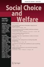
For any three-member jury on two equally likely states of Nature, if its ability set has a homogeneity index at least 6/7, then the reliability of simultaneous honest voting is at least that of sequential honest voting. On the other hand, if its ability set has a heterogeneity index at least 4/3, then the reliability of sequential voting in the optimal order is at least that of simultaneous voting.
The results in Theorem 5 can be illustrated in Fig. 1, in which we set the middle ability \(b=1/2\) and consider the square \((a,c)\in [0,1/2]\times [1/2,1]\). The curved line divides this square into two regions, where sequential (top-left) and simultaneous (bottom-right) voting are optimal. Within these two regions are the respective rectangles where Theorem 5 guarantees simultaneous voting is better (\(\lambda \ge 6/7\)) and where sequential voting is better (\(\mu \ge 4/3\)). Note that when \(b=1/2\), the condition \(\lambda \ge 6/7\) corresponds to rectangle \(\{(a,c): a\ge 3/7, c\le 7/12\}\), while condition \(\mu \ge 4/3\) corresponds to rectangle \(\{(a,c): a\le 3/8, c\ge 2/3\}\).
Fig. 1
Comparison of majority voting scheme: Simultaneous vs. sequential
×
Remark 4
Theorem 5 shows that, when a jury is highly homogeneous, simultaneous voting helps diversify the homogeneity. On the other hand, when a jury is highly heterogeneous, sequential voting helps unify the heterogeneity. Interestingly, our above theorem seems consistent with the result for simultaneous voting obtained by Ben-Yashar and Nitzan (2017) in that high reliability of simultaneous voting needs homogeneity, while diversity calls for sequential voting. Ben-Yashar and Nitzan (2017) show that when adding voters to a jury to increase its reliability, homogeneity is useful.
9.5 Diversity for reliability
We can now answer the question of whether homogeneous or heterogenous juries have higher reliability under sequential honest majority voting. Kanazawa (1998) has shown that the reliability of Condorcet simultaneous voting of a jury, with fixed average of the abilities of the jurors, is increasing in the standard deviation of juror abilities. Here, we show that this is similarly true in terms of heterogeneity and homogeneity indices, and sequential voting.
Theorem 6
Under honest majority voting on two equally likely states of Nature, fixing the average ability of any three-member jury, reliability is a strictly increasing (resp. decreasing) function of the heterogeneity (resp. homogeneity) index. In other words, high heterogeneity (resp. homogeneity) of jurors’ abilities helps (resp. harms) reliability.
According to Theorem 5, simultaneous voting can have higher reliability than sequential under honest voting. This cannot occur under strategic voting, since the jurors could ignore prior voting and thus achieve the reliability of simultaneous voting. The next theorem provides a sufficient condition for achieving strategic optimality (see Sect. 9.1).
Theorem 7
Given equally likely states of Nature, sequential honest voting (in optimal order) achieves strategic optimality if heterogeneity of the jurors’ abilities is at least 7/4, while simultaneous honest voting achieves strategic optimality if the jurors all have the same ability.
Note that strategic optimality in our model is a benchmark for measuring the quality of a majority verdict. In the work by Dekel and Piccione (2000), it is assumed that all jurors care about the correctness of the jury verdict, which is in contrast to the assumption in our model that they each care about the correctness of their own votes.
9.7 Sequential deliberation
In our voting model, we assume that signals are private information. In some applications, information exchange, which we call deliberation, is possible and individuals reveal private information in some order, which lets the quality of judgments increase. The question arises as to what the optimal order in deliberation should be, which we answer in this subsection.
We refer the following model as sequential deliberation: When each juror votes in our original sequential voting model, the voting juror is required to reveal his signal in addition to his vote. More specifically, given a jury of n jurors of abilities \(a_1, \ldots , a_n\) and a priori probability \(\theta\) for \(N=A\), by (honest) sequential deliberation of the jury in sequence \({\varvec{a}}=(a_1, \ldots , a_n)\), we mean that, for \(m=1, \ldots , n\), the juror in position m receives signal-ability pairs \((s_i, a_i)\), \(i=1, \ldots , m\), and then votes \(v_m=A\) if \(\Theta \ge 1/2\) and \(v_m=B\) otherwise, where \(\Theta \equiv \Theta \left( \theta , (s_1,a_1), \ldots , (s_k, a_m)\right)\) is the posterior probability of \(N=A\) associated with information of \(\{(s_1, a_1) \ldots , (s_m, a_m)\}\). In fact, using Bayesian update (4) repeatedly, we can obtain for any \(n\ge 1\):
where \(\pi _i=s_i a_i\), and \(\zeta (i)=1\) if i is odd, \(\zeta (i)=0\) otherwise, \(i=1,\ldots ,n\). The following theorem provides an answer to optimal sequencing in sequential deliberation, where jurors sequentially reveal their signals (and the associated votes).
Theorem 8
For sequential deliberation of any odd-size jury of known abilities, the probability of a correct majority verdict is maximized by the seniority ordering.
Up to now we have considered the optimal voting order problem only for juries of size three, where we have the definitive result Theorem 2. For larger juries we only know the optimal ordering for the last two jurors (decreasing ability, see Theorem 1) and we have some numerical results comparing the seniority order (SO) with the anti-seniority order (AO) in Sect. 8, namely, the former is more likely to be correct when the verdicts differ. For larger juries the “curse of dimensionality” prevents us from using the earlier technique of deriving a formula for the reliability of a jury with a given order of abilities because the number of thresholds increases exponentially in the jury size. So in this section we will use simulation to estimate this reliability, by generating many random signal vectors for a given ability order jury, assuming one of the alternatives (say A) holds. For each, we compute the verdict. Finally, we estimate reliability as the fraction of verdicts which are correct (in this case, A).
In general, we cannot consider all possible orderings (permutations) of a set of abilities. In addition to SO and AO, we propose a new ordering which we call the Ascending-Descending Order (ADO). For a jury of odd size \(n=2m+1\), this ordering begins with the most able \(m+1\) jurors voting in increasing (anti-seniority) order and then has the m least able jurors voting in descending (seniority) order. In particular, the median ability juror votes first, the highest ability juror votes in the median position and the least able juror votes last.
Definition 2
Given a set of \(n=2m+1\) distinct abilities indexed in increasing order \(0 \le a_{1}<a_{2}<\dots <a_{n}\le 1\), the Ascending-Descending Order (ADO) is given by
Note that for \(n=3\) our main result, Theorem 2, says that the ADO is the unique optimal ordering. Furthermore, ADO has its last two jurors voting in decreasing order, which is a requirement of any optimal ordering according to Theorem 1. Our simulations, admittedly limited in number, have not yet produced any counter-examples to the following.
Conjecture 1
For any fixed set of an odd number of distinct abilities for a jury, the ordering that produces the highest reliability is the ADO.
Of course we have already proved the conjecture for juries of size three in Theorem 2. Even if the ADO turns out to not always be optimal, our simulation results seem to show that it a good heuristic, producing high reliabilities.
Our first simulation is concerned with a jury of size five, which we take as the ability set \(\{0.1,0.3,0.5,0.7,0.9\}\), which is in some sense uniformly distributed. For simplicity, we denote them by \(\{1,3,5,7,9\}\) for the rest of this section. If two abilities are very close, then transposing the voting order of the two corresponding jurors would not greatly affect the reliability, and the difference might be less than the error in the simulation. There are \(5!=120\) orderings of such a jury, but only 60 for which the last two abilities are in decreasing order. We calculated 100,000 random signal vectors (generated from alternative A) for each such ordering and counted the number of (correct) verdicts for A, this number divided by 100,000 is an estimate of reliability. Of these 60, exactly 9 had an estimated reliability \({\hat{\rho }}\) above 76%. We then calculated 1,000,000 trials for these, listing the results in Table 2 below. The estimates have error less than 0.1% with a confidence of 90%. Note that ADO has the highest estimated reliability, at 77%.
Table 2
Estimated reliability of five-member juries
Voting order
No. of A verdicts
Est. reliability \({\hat{\rho }}\) (%)
(5,7,9,3,1)
770,199
77.0
(7,5,9,3,1)
766,450
76.6
(1,7,9,5,3)
762,953
76.3
(7,3,9,5,1)
762,488
76.2
(7,9,1,5,3)
762,437
76.2
(5,9,7,3,1)
762,326
76.2
(7,9,5,3,1)
762,186
76.2
(7,9,3,5,1)
761,472
76.1
(7,1,9,5,3)
761,321
76.1
The increasing order (1, 3, 5, 7, 9) (AO) had \({\hat{\rho }}=71.5\%\); the decreasing order (9, 7, 5, 3, 1) (SO) had \({\hat{\rho }}=75.5\%\); the ordering with the lowest estimated reliability was (5, 3, 1, 9, 7) with \({\hat{\rho }}=64.2\%\). It is worth noting that there is more than a 10% difference in reliability between ADO and the worst ordering.
To look at seven-member juries, it is no longer feasible to check the reliability of all \(7!/2=2520\) orderings even of a particular set of abilities. Instead, we generated 500 random juries \(\mathbf {a}\) (independently picking each juror with an ability uniformly in [0, 1]). For each, we calculated the estimated reliability \({\hat{\rho }}(\mathbf {a})\) and \({\hat{\rho }}^{*}(\mathbf {a}^{*})\), where \(\mathbf {a}^{*}\) is the reordering of \(\mathbf {a}\) to ADO. For example, if \(\mathbf {a}=(0.3,0.6,0.4,0.1,0.8,0.5,0.7)\) then \(\mathbf {a}^{*}= (0.5,0.6,0.7,0.8,0.4,0.3,0.1)\). We used 10,000 trials for each randomly generated jury \(\mathbf {a}\), and calculated the difference \({\hat{\Delta }}(\mathbf {a}) = {\hat{\rho }}^{*}(\mathbf {a})-{\hat{\rho }}(\mathbf {a})\) between reliability in ADO order and in the originally generated order. The mean value of \({\hat{\Delta }}\) was 0.036969 (roughly a \(4\%\) improvement in the reliability of the verdict), the maximum was 0.1609 (a \(16\%\) improvement in reliability) and the minimum was \(-0.0064\). The frequency distribution is given in Table 3 (no data at boundary points).
Table 3
Frequency distribution of \({\hat{\Delta }}\)
Range
(\(-\) 0.02,0)
(0,0.02)
(0.02,0.04)
(0.04,0.06)
(0.06,0.08)
Frequency
10
139
171
94
45
Range
(0.08,0.10)
(0.10,0.12)
(0.12,0.14)
(0.14,0.16)
(0.16,0.18)
Frequency
20
14
6
0
1
So from the heuristic point of view, it certainly seems a good idea to rearrange a jury (of size 7), which arrives in random order, into one in ADO order, if this is allowed. It nearly always gives an improvement in reliability. From the theoretical point of view, it at first may appear that we have found ten counter-examples to our Conjecture 1 regarding the optimality of ADO, in that the original order of the jurors that produced a negative \({\hat{\Delta }}\) is more reliable than ADO. However, the negative values were very close to zero. There were 11 juries \(\mathbf {a}\) where \({\hat{\Delta }}(\mathbf {a})<0.001\) and we recalculated \({\hat{\Delta }}\) for all of them with one million trials. All came out with a positive value of \({\hat{\Delta }}\). There was one additional jury \(\mathbf {a}\) for which \({\hat{\Delta }}(\mathbf {a})\) was not negative but was less than 0.001. We also recalculated this for one million trials and checked that it still came out positive.
Despite the aforementioned efforts, the search for a counter-examples to Conjecture 1 is far from exhaustive.
Another way of evaluating the ADO is to compare it to SO (Seniority, or Descending Order), in the same way we compared SO to AO in Sect. 8. For odd values of \(n=5, 7, 9, 11\) , we generate one million random juries with associated random signals generated, assuming Nature is A. We record in Table 4 (with the same notation as in Table 1) the number of verdict pairs for ADO and SO, respectively, and determine the probability that ADO is the correct verdict (that is, A) when the two verdicts differ.
Table 4
Relative performance of jury orderings: ADO and SO
Jury size n
#(B,B)
#(A,A)
#(A,B)
#(B,A)
R (%)
5
150631
656425
101988
90956
53
7
117189
682142
107038
93631
53
9
94630
702166
109739
93465
54
11
78453
719629
110279
91639
55
From Table 4, we see that when ADO and SO give different verdicts, ADO is the correct one about 53% of the time for juries of size five, rising to about 55% of the time for juries of size 11.
11 Concluding remarks
When jurors of differing abilities vote sequentially, the reliability of the majority verdict depends on the voting order. We have shown that, regardless of the set of abilities on a three-member jury, if the two states are equally likely, then the optimal voting order is always median ability first, then highest ability, then lowest ability. The optimality of the ordering is robust for the a priori probability \(\theta\) around 1/2.
Our earlier paper, Alpern and Chen (2017a) showed that this was true for many ability sets, but this is the first paper to establish this result rigorously for all ability sets. Analogous results for larger juries appear to be beyond current methods, but presumably special cases could be studied, for example, when only one juror has a different ability than the others.
Since the optimal ordering is established, we can fix this ordering and then make various reliability comparisons. To do this, we have defined indices that measure homogeneity and heterogeneity of the set of jurors. We find that for sufficiently homogeneous juries, simultaneous voting is more reliable than sequential voting. On the other hand, when juries are sufficiently heterogeneous, sequential voting is more reliable. In a similar vein, we find that the reliability of a jury of fixed average ability is increasing in its heterogeneity. For sufficiently heterogeneous juries, the thresholds given by honest voting are in fact the optimal joint thresholds, so that honest voting optimizes the reliability of the majority verdict. That is, honest voting is also strategic.
For larger juries, we have introduced the Ascending–Descending Order of voting and shown that it is at least an excellent heuristic for obtaining high reliability, if not actually optimal. Further work in this direction for large juries would be useful, including asymptotic results analogous to those of Condorcet.
Open AccessThis article is licensed under a Creative Commons Attribution 4.0 International License, which permits use, sharing, adaptation, distribution and reproduction in any medium or format, as long as you give appropriate credit to the original author(s) and the source, provide a link to the Creative Commons licence, and indicate if changes were made. The images or other third party material in this article are included in the article's Creative Commons licence, unless indicated otherwise in a credit line to the material. If material is not included in the article's Creative Commons licence and your intended use is not permitted by statutory regulation or exceeds the permitted use, you will need to obtain permission directly from the copyright holder. To view a copy of this licence, visit http://creativecommons.org/licenses/by/4.0/.
Publisher's Note
Springer Nature remains neutral with regard to jurisdictional claims in published maps and institutional affiliations.
As in Sect. 5.5.1, we let \(0\le b < c\le 1\) be the jurors’ abilities and A be the designated favored alternative (i.e., B be the alternative needing unanimous vote). Denote by \(\theta\) the a priori probability of A and by \({\bar{Q}}(\theta ; b,c)\) the reliability of the jury verdict. Using the last equation in (16), we compute \({\bar{Q}}(\theta ; b,c)\) for any \(\theta \in [0,1]\) and any \(b,c\in [0,1]\). We then prove that \({\bar{Q}}(\theta ; c,b) - {\bar{Q}}(\theta ; b,c)\ge 0\) when \(c \ge b\). To this end, we use Wolfram Mathematica, a mathematical symbolic computation program, with its command FullSimplify[expr,assum], where expr is replaced by expression \({\bar{Q}}(\theta ; c,b) - {\bar{Q}}(\theta ; b,c)\ge 0\) and assum is replaced by constraints \(c > b\) and \(\theta ,b,c\in [0,1]\). The command outputs True in a couple of seconds. Alternatively, we also use command FindInstance[expr,vars], where expr is replaced by the system of inequalities \({\bar{Q}}(\theta ; c,b) - {\bar{Q}}(\theta ; b,c)< 0\), \(c > b\) and \(\theta , b,c\in [0,1]\), while vars is replaced by the specification of variables \(\{\theta ,b,c\}\). The command outputs the empty set \(\emptyset\) (i.e., there is no solution to the system) in a couple of seconds. The reader is referred to Section 3.1 of Chen (2021), where details of the aforementioned computation are provided.
In the remainder of the Appendix, wherever we use Mathematica in the aforementioned ways for an algebraic proof of an inequality subject to some (inequality) constraints, we will simply refer the reader to the location in Chen (2021) for details, as we do above.
As explained in Appendix 12.1 above, for proving inequality of \(f_1(a,b,c)>0\) with constraints \(a,b,c\in [0,1]\), \(\rho (b,a)<c\le \rho (a,b)\) and \(b/2<a <b\), see Section 3.2 of Chen (2021) for details.
Part 2
Now consider \(c > \rho (a,b)\). If \((b,a,0)\in H_2\), then
$$\begin{aligned} \Delta _1(a,b,c) =q(a,b,c)-\frac{b+2}{4} = \frac{f_2(a,b,c)}{128 b c (8-a^2-2 a b)}, \end{aligned}$$
where
$$\begin{aligned} f_2(a,b,c) =&-4 (a - 2 b)^3 + 4 \left( 8 - a^2 - 2 a b\right) \left( a^2 + 4 a b - 4 b^2\right) c \\&\; + (2 b-a) \left( 8 - a^2 - 2 a b\right) ^2 c^2. \end{aligned}$$
As a convex quadratic function of c, \(f_2(a,b,c)\) is minimized at
$$\begin{aligned} c_1=\frac{2 \left( 4 b^2-a^2-4 a b\right) }{(2 b-a) \left( 8-a^2-2 a b\right) } \end{aligned}$$
to
$$\begin{aligned} f_2(a,b,c_1)=\frac{64 a^2 b (b-a)}{2b-a} > 0. \end{aligned}$$
If \((b,a,0)\not \in H_2\), then it is easy to check that \(\rho (a,b)>\rho (b,a)\) and hence \(c> \rho (a,b)>\rho (b,a)\). We obtain
$$\begin{aligned} \Delta _1(a,b,c) = q(a,b,c)-q(b,a,c)=\frac{(b-a) f_3(a,b,c)}{128 a b c \left( 8-2 a b-a^2\right) \left( 8-2 a b-b^2\right) }, \end{aligned}$$
where
$$\begin{aligned} f_3(a,b,c)&= c^2(a+b)\left( 8-2 a b-a^2\right) \left( 8-a^2-b^2\right) \left( 8-2 a b-b^2\right) \\&\quad -4 c\left( 8-2 a b-a^2\right) \left( a^2+a b+b^2\right) \left( 8-2 a b-b^2\right) \\&\quad -4(a+b)\left( 10 a^3 b-7 a^2 b^2-8 a^2+10 a b^3-16 a b-8 b^2\right) , \end{aligned}$$
which is positive under constraints \(c> \rho (a,b)\) and \(b/2< a < b\) with \(a,b,c\in [0,1]\) [Section 3.3 of Chen (2021)].
According to (19), if \(c\le a/2\), then \(c<b/2\), we have \(\Delta _2(a,b,c) \equiv Q(b,c,a) - Q(a,c,b)=(b-a)/4 >0\). If \(a/2 <c\le b/2\), then according to (13), \(b>\rho (a,c)\), which leads to
which is positive under constraints \(a/2 <c\le b/2\) and \(a,b\in [0,1]\) [Section 3.4 of Chen (2021)]. Therefore, we only need to consider \(c > b/2\). If \(a \le \rho (b,c)\) and \(b \le \rho (a,c)\), then
To prove the stated monotonicity of Q(a, b, c) in a, b, c respectively, we only need to do so for each of the three pieces of Q(a, b, c) in (19) thanks to the continuity of Q(a, b, c) over \(a,b,c\in [0,1]\). The stated monotonicity of \(Q(a,b,c)\equiv (2+a)/4\) is evident over domain \(H_2\). We show that \(q_0(a,b)\) and q(a, b, c) have the stated monotonicity over \(H_3\) and S, respectively. We accomplish this by verifying [Section 3.7 of Chen (2021)] that each of the following two partial derivatives
Let homogeneity index \(\lambda (a,b,c)\ge 6/7\). Then with formulae derived in Sect. 9.2, we have
$$\begin{aligned} Q_{\text {sim}}\left( {\textstyle \frac{1}{2}},a,b,c\right) - Q(b,c,a) = \frac{h_1(a,b,c)}{128 a c \left( 8-2 b c-b^2\right) }, \end{aligned}$$
where
$$\begin{aligned} h_1(a,b,c)&= 64 a^2 b - 32 a b^2 + 4 b^3 - 16 a^2 b^3 + 4 a b^4 + a^2 b^5 \\&\quad - 24 b^2 c - 16 a^2 b^2 c + 8 a b^3 c + 2 a^2 b^4 c + 48 b c^2 - 32 c^3, \end{aligned}$$
which is non-negative when \(\lambda (a,b,c)\ge 6/7\) [Section 3.8 of Chen (2021)]. On the other hand, let the heterogeneity index \(\mu (a,b,c)\ge 4/3\), then we have
$$\begin{aligned} Q(b,c,a)-Q_{\text {sim}}\left( {\textstyle \frac{1}{2}},a,b,c\right) = \left\{ \begin{array}{ll} {\displaystyle \frac{h_2(a,b,c)}{32c}}, &{} \text{ if } a \left( b^2+2 b c-8\right) +4 c\ge 2 b; \\ {\displaystyle \frac{-h_1(a,b,c)}{128 a c \left( 8-2 b c-b^2\right) }}, &{} \text{ otherwise }; \\ \end{array} \right. \end{aligned}$$
where
$$\begin{aligned} h_2(a,b,c) = b c (a c-4)+4 c (c-a)+2 b^2. \end{aligned}$$
Both \(h_2(a,b,c)\) and \(-h_1(a,b,c)\) are non-negative when \(\mu (a,b,c)\ge 4/3\) with the former non-negativity having the additional constraint \(a \left( b^2+2 b c-8\right) +4 c\ge 2 b\) [Section 3.9 of Chen (2021)].
Let us first focus on heterogeneity. Fix \(m\in (0,1)\) as the average ability of the jury. Then the three abilities can be expressed as functions of m and the heterogeneity index \(\mu\) as follows:
Then the following function \({\bar{Q}}(m,\mu )\), with \(0\le m\le 1\) and \(\mu \ge 1\), is the reliability of honest majority voting by the jury with optimal voting sequence:
For any fixed \(m \in (0,1)\), function \(w(m,\mu )\) in domain \(\{\mu \ge 1: w(m,\mu )\ge 0\}\) and functions \({\bar{Q}}_1(m,\mu )\) and \({\bar{Q}}_2(m,\mu )\) in domain \(\{\mu : \mu \ge 1\}\) are all strictly increasing, which can be shown by verifying that the relevant partial derivatives are positive under corresponding constraints [see Section 3.10 of Chen (2021)}. Similarly, we can shown that, if \(1\le \mu _1< \mu _2\) and \(w(m,\mu _1)<0\le w(m,\mu _2)\), then
Combination of these facts implies that \(Q(m,\mu )\) is strictly increasing in \(\mu \ge 1\) for any fixed \(m \in (0,1)\).
Now let us discuss homogeneity. Similar to our above definitions of \({\bar{a}}(m,\mu )\), \({\bar{b}}(m,\mu )\) and \({\bar{c}}(m,\mu )\), the three abilities can be expressed as functions of m and the homogeneity index \(\lambda\) (\(0<\lambda \le 1\)) as follows:
the required monotonicity (strict decrease in \(\lambda\)) of \({\tilde{Q}}(m,\lambda )\) follows from the monotonicity (strict increase in \(\mu\)) of \({\bar{Q}}(m,\mu )\).
Let heterogeneity index \(\mu (a,b,c)\ge \frac{7}{4}\). Then reliability of sequential honest voting is \(Q(b,c,a)=q_0(b,c)\) according to (19). Since \(Q_{\text {str}}\) is clearly non-decreasing in a, with \(a\le \frac{4}{7} b\) we conclude that the difference of the two reliabilities is at least
We show that \(\Omega\) is non-negative when \(d=c\), from which and (20) the first part of the theorem follows. Note that the coefficient of \(d^2\) in the \(\Omega\) function is non-negative. Therefore, \(\Omega\) is lower bounded by its value at \(d=0\):
where \(\mu \equiv c/b\ge 7/4\). We can show that \(\Omega (b,c,0, y_1, y_2, z_1, z_2)\ge 0\) subject to \(\mu \ge 7/4\) and \(y_1, y_2, z_1, z_2\in [-1,1]\) [Section 3.11 of Chen (2021)].
The second part of the theorem follows from (20) and the fact that (Section 3.12 of Chen (2021)):
Given any a priori probability\(\theta\)of\(N=A\), the probability\(P(\theta ,a)\)of an honest juror of abilityavoting correctly isnon-decreasing in\(a\in [0,1]\).
Proof
The honest threshold of the juror is \(\tau _a(\theta )\) given in (5) in Sect. 5.1. The probability that the juror votes correctly is the probability that his signal \(s\ge \tau _a(\theta )\) when \(N = A\) plus the probability that \(s < \tau _a(\theta )\) when \(N = B\). That is,
Now let us prove Theorem 8 by establishing the following theorem, which implies Theorem 8 by setting \(m=(n+1)/2\).
Theorem 9
For sequential deliberation of anyn-member jury of known abilities and any\(m \in \{1,\ldots , n\}\), the probability of at leastmcorrect votes is maximized by the seniority ordering.
Proof
Given any a priori probability \(\theta\) of \(N=A\), let \({\varvec{a}}=(a_1, \ldots , a_n)\) be a sequence of abilities for sequential deliberation that maximizes the probability of at least m correct votes, and let \({\varvec{v}}=(v_1, \ldots , v_n)\) be the sequence of the corresponding deliberation votes. If \({\varvec{a}}\) is not a seniority ordering, then there is k (\(1\le k < n\)), such that \(a_k < a_{k+1}\). Consider the new deliberation sequence \({\varvec{a}}'=(a_1, \ldots , a_{k-1}, a_{k+1}, a_k, a_{k+2}, \ldots , a_n)\), which is the same as \({\varvec{a}}\) except that the order of jurors in positions k and \(k+1\) are swapped. Let \({\varvec{v}}'=(v_1', \ldots , v_n')\) be the corresponding deliberation votes. Then it is clear that \(v_i'=v_i\) for \(i=1, \ldots , k-1, k+1, \ldots , n\), since each pair of these votes, \(v_i'\) and \(v_i\), use the same set of signal-ability pairs for their posterior probability \(\Theta\) of A, which uniquely determines their deliberation votes. In other words, \({\varvec{v}}\) and \({\varvec{v}}'\) can differ only in their kth components, \(v_k\) and \(v_k'\).
The two orderings \({\varvec{a}}\) and \({\varvec{a}}'\) differ in having at least m correct votes only if they have at least \(m-1\) correct votes not counting the kth vote. So the only thing that matters is the probability of the kth vote being correct. We now show that it is more likely to be correct for \({\varvec{a}}'\). Denote \(\theta '=\Theta \left( \theta , (s_1,a_1), \ldots , (s_{k-1}, a_{k-1})\right)\), the posterior probability of A associated with information \(\{(s_1,a_1), \ldots , (s_{k-1}, a_{k-1})\}\). Then we have that the probabilities of \(v_k\) and \(v_k'\) being correct are \(P(\theta ', a_k)\) and \(P(\theta ', a_{k+1})\), respectively. According to Lemma 2, \(P(\theta ', a_k)\le P(\theta ', a_{k+1})\) since \(a_k < a_{k+1}\). □
Mathematica computations
This section provides pointers to the locations in Chen (2021), a Wolfram Mathematica Notebook, where details are provided for all the algebra from equation (19) onwards that Mathematica helps with. Those to the left of the colon symbols below are locations in the paper with natural sequence of their appearances and to the right are the corresponding locations in Chen (2021).
Equation (19): Section 1.2.1 “Reliability Q with equiprobable alternatives”.
Section 7.1, expression \(f_1(a,b,c)\): Item 1 of Section 2.1 “Order of the first two voters”.
Section 9.1, expression \(Q_{\text {str}}({\textstyle \frac{1}{2}}, a,b,c, x, y_1, y_2, z_1, z_2)\): Section 1.4 “Reliability function of sequential strategic voting”.
Appendix 12.2, expressions \(f_2(a,b,c)\) and \(f_3(a,b,c)\): Items 2 and 3 of Section 2.1 “Order of the first two voters”.
Appendix 12.3, expressions \(f_4(a,b,c)\) and \(f_5(a,b,c)\): Section 2.2 “Order of the two end-voters”.
Appendix 12.5, expressions \(h_1(a,b,c)\) and \(h_2(a,b,c)\): Section 1.5 “Reliability function of simultaneous honest voting” and Section 2.3 “Sequential versus simultaneous majority voting”.
Appendix 12.6, expressions \(w(m,\mu )\), \(u(m,\mu )\) and \(v(m,\mu )\): Section 2.4 “Reliability versus heterogeneity and homogeneity”.
Appendix 12.7, expressions \(\Omega (b,c,d,y_1, y_2, z_1, z_2)\) with \(d=c\): Section 2.5 “Strategic optimality versus heterogeneity and homogeneity”.
We use Wolfram Mathematica, a mathematical symbolic computation program, for all the straightforward but tedious algebraic calculations onwards. See Appendix 12.9 for more details.